- SAP Community
- Products and Technology
- Technology
- Technology Blogs by SAP
- Automate your Excel to Datasphere upload
- Subscribe to RSS Feed
- Mark as New
- Mark as Read
- Bookmark
- Subscribe
- Printer Friendly Page
- Report Inappropriate Content
Introduction
SAP Datasphere is SAP's next-generation cloud data warehouse solution. It's a great foundation for your business's data landscape, allowing you to easily integrate both SAP and non-SAP data from live systems and local files into a single system. Your data will be stored in tables and transformed using views and models
At the beginning of a Datasphere project, it's possible that a connection to source systems like S/4 HANA or Business Warehouse hasn't been established yet. However, often it's still important to create an initial proposal to present a customer-specific Datasphere use-case. In this situation, you can upload Excel or CSV files to the system and use them as a data source for the proposal. For a general guideline on how to upload Excel files to SAP Datasphere, please refer to this Tutorial. Creating multiple tables and their relations from flat files can be a tedious task, especially in larger proposals or bigger projects.
This blog post presents a quick and simple method for automatically uploading all dimension and fact tables simultaneously. The appropriate data type and length for all columns is selected and associations between the fact and dimension tables are created automatically, all in one step.
This is achieved by accelerating the capabilities of the JSON/CSN to Entity Relationship Model (ERM) feature in SAP Datasphere. The JSON structure represents all local dimension and fact tables with their associations and is automatically generated using a Python script. Just running the script once creates the JSON file that can then be uploaded to Datasphere as an ERM. Uploading and saving the ERM creates the structure of local tables and relations in Datasphere.
Supported capabilities
- Automatic table generation from local files
- CSV and Excel file data sources
- String, Integer, Decimal, and Date column data types
- Different string and decimal lengths
- Key columns for dimension tables
- Differentiating between Fact and Dimension tables using star schema
- Simple associations (one-column) between Fact and Dimension tables
Not supported
- Multicolumn associations
- Snowflake schema (associations between dimensions)
- Assigning semantic types and label columns to columns
- Hierarchies
This blog post explains the basic functionality using a smaller example. However, the proposed solution is particularly valuable when working with a large number of tables, as demonstrated in this demo:
Table of Contents
3.2 Prerequisites Regarding Files and File Structure
5.2 Uploading JSON to Datasphere
Quick Note: If you want to quickly start uploading the CSV files to Datasphere, you can refer to this link to download the complete Python script. Follow the instructions in the prerequisites and application section.
Basic Concepts
- JSON/CSN: JSON (JavaScript Object Notation) is a lightweight data interchange format that is readable by both people and machines. It consists of key-value pairs and ordered lists of values, known as arrays. CSN is a schema notation that expands JSON's capabilities and can be used to build Entity Relationship Models (ERMs). For available definitions, refer to this link.
- Entity Relationship Model (ERM): ERMs represent a specific domain of knowledge. They are diagrams that organize entities (tables) and their relationships. In Datasphere, ERMs are used to represent or create the structure of tables and views within the system. For further information, see this link.
- Python, Pandas, and Numpy: Python is one of the most widely used programming languages known for its readability. It is commonly used for various tasks, including data transformation and preparation. Pandas and Numpy are libraries within Python that allow you to work with tables and provide many basic functionalities when working with data.
Data Explanation
For this blog, a simple example is chosen to explain the basic application of creating a JSON structure file from the remote tables and uploading it to Datasphere. However, the proposed script works flexibly with different business domains and a different number of files.
This example contains only three tables: one fact table with headcount information per organizational unit and grade level, and two dimension tables. One dimension table contains the organizational units, and one table contains grade levels with additional information.
Fact Table:
Dimension Tables:
Grade Dimension
Legal Entity Dimension
Recognise that the column names in the fact and dimension tables are not the same, but the columns will still be mapped in the process. In addition there are different data types in the tables that will be automatically detected.
Prerequisites
There are some prerequisites regarding the technical setup and others regarding file structure and format.
Technical Setup
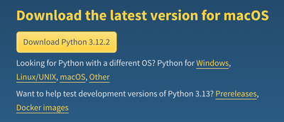
The code is written in Python, so you will need a Python environment to run it. If you haven't installed one yet, you can download Python for Windows, Mac, or Linux from the official Python website here. Make sure to download a version > 3.7 for optimal compatibility. Once downloaded, run the Python installer and accept all default settings. For further assistance, refer to the official documentation here.
The Python environment comes with the pip command-line tool, which you can use to install additional libraries. To run the proposed code, you will need to install two additional libraries: Pandas and Numpy. You can easily install them by running these two commands from the command line.
$ pip install numpy
$ pip install pandas
Additionally JSON and os libraries are needed and imported in the beginning of the script. However, these are preinstalled with Python and therefore do not need to be installed with Pip. That is all for the technical setup. Now you need to organise your files in a way they are understood by the script.
Files and File structure
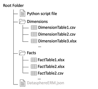
To upload data to Datasphere, you can use CSV or Excel (.xlsx) files, or both. It's important to note that the primary key, which is referenced by the fact tables, must be the first column in the dimension tables. To ensure that the script can find the respective files, it's necessary to follow a specific file structure. You should place each Dimension Table in a subfolder called 'Dimensions' and each Fact Table in a subfolder called 'Facts'. Make sure that your Python script file is in the same location as the two folders. The JSON file that is generated will also be created in the same location as the script file. To summarize, your file structure should look like this:
Please be aware that on Mac, a hidden file called “.DS_Store” may be automatically generated within the folders. This file stores custom attributes of a folder and can be deleted with the following command in the respective folder:
$ find . -name ".DS_Store" -delete
Now you are all set to start generating your JSON file. If you're not interested in the code, feel free to skip the explanation and jump right into the application.
Code Explanation
This section provides a brief explanation of how the JSON file is generated from local tables. It assumes a basic understanding of programming concepts such as loops, functions, and datatypes. The code presented here is not complete, but it highlights the most important ideas. To obtain the complete file, please refer to the download link provided here instead of copying the code manually.
1 Imports
Some build in and additional libraries are needed. They are imported in the beginning. How to install numpy and pandas is explained in the prerequisites.
import os
from os.path import isfile, join
import numpy as np
import pandas as pd
import re
import json
2 Read CSV/Excel files
The function reads fact and dimension tables and stores them in two dictionaries: 'facts' and 'dims', which are then returned. To achieve this, it first reads the current working directory and retrieves the fact table names from the 'Facts' subfolders and the dimension table names from the 'Dimensions' subfolder. Only CSV and XLSX files are supported, which are read as a Pandas dataframe and added to the respective dictionary. If there are any other file types in the subfolders, an exception is raised.
def get_csv_names():

    current_path = os.getcwd()

    #Fact Tables are defined in the path ./Facts
    factpath = current_path + "/Facts"
    factnames = [f for f in os.listdir(factpath) if isfile(join(factpath, f))]

    #Creating a fact-dictionaly of filename : file
    facts = {}
    for file in factnames:
        print(file)
        if file.split(".")[1] == "csv":
            facts[file[:-4]] = pd.read_csv(factpath+"/"+file)
        elif file.split(".")[1] == "xlsx":
            facts[file[:-5]] = pd.read_excel(factpath+"/"+file)
        else:
            raise Exception(f"can not return json because the following fields could not be assigned: {file}")

    #Dimensions Tables are defined in the path ./Dimensions
    dimpath = current_path + "/Dimensions"
    dimnames = [f for f in os.listdir(dimpath) if isfile(join(dimpath, f))]

    #Creating a dimension-dictionaly of filename : file
    dims = {}
    for file in dimnames:
        print(file)
        if file.split(".")[1] == "csv":
            dims[file[:-4]] = pd.read_csv(dimpath+"/"+file)
        elif file.split(".")[1] == "xlsx":
            dims[file[:-5]] = pd.read_excel(dimpath+"/"+file)
        else:
            raise Exception(f"can not return json because the following fields could not be assigned: {file}")
    return facts, dims
3 Build JSON
3.1 Initalize the JSON
The beginning and end of JSON files always define meta-data and are not dependent on the tables themselves. The JSON object is a nested Python dictionary that is later dumped into a JSON file.
def build_json():

    facts, dims = get_csv_names()

    #Initalize JSON structure
    json = {
        "definitions": {},
        "version": {
            "csn": "1.0"
        },
        "meta": {
            "creator": "ER Modeler",
            "kind": "sap.dwc.ermodel",
            "label": "PeopleTemplate"
        },
        "$version": "1.1"
    }
3.2 Add Table definition
The script iterates over every fact (and later dimension) table retrieved from the get_csv_names() function. The Table is added to the definitions of the json object. The structure slightly varies between fact and dimension tables. The tablename is put in as a variable.
for tablename, table in facts.items():

    # Setting up JSON structure for each fact table
    json["definitions"][tablename] = {
      "kind": "entity",
      "@EndUserText.label": tablename,
      "@ObjectModel.modelingPattern": {
          "#": "ANALYTICAL_FACT"
      },
      "@ObjectModel.supportedCapabilities": [
          {
          "#": "DATA_STRUCTURE"
          }
      ],
      "@DataWarehouse.pinToMemory": True,
      "elements":{}
    }
3.3 Add columns with datatypes
The JSON includes a separate object for each column in a table, located within the elements section of the table definition. The structure of each object varies depending on the datatype (e.g. string, integer, etc.), with support limited to string, integer, decimal, and date. Pandas automatically detects the datatypes when reading the CSV/Excel file so they only need to be mapped here. For decimal and string the length is automatically retrieved. The code is slightly different for dimension columns, since no measure types are defined, but a key column is specified.
# Iterating through columns in facts
for column, dtype in zip(table.columns[start:], table.dtypes[start:]):
    # Handling different data types
    if dtype == np.int64:
        # Handling integers
        json["definitions"][tablename]["elements"][column] = {
            "type":"cds.Integer"
						"@AnalyticsDetails.measureType": {
                "#": "BASE"
            },
            "@Aggregation.default": {
                "#": "SUM"
            }
        }
    elif dtype == np.float64 or dtype== np.float32:
        # Handling floating point numbers
        if str(max(table[column])) != "nan":
            precision, scale = [len(w) for w in str(max(table[column])).split('.')]
            precision += scale
            if scale == 0:
                scale = 1
        else:
            precision = 15
            scale = 3
        json["definitions"][tablename]["elements"][column] = {
            "type":"cds.Decimal",
            "precision":precision,
            "scale":scale,
						"@AnalyticsDetails.measureType": {
                "#": "BASE"
            },
            "@Aggregation.default": {
                "#": "SUM"
            }
        }
    elif dtype == np.object0:
        # Handling strings/object types
				if check_date(table, column, dtype):
            #Handling Date
            json["definitions"][tablename]["elements"][column] = {
                "type":"cds.Date"
            }

				else:
          chars = 0
          for i in table[column]:
              chars = max(chars, len(str(i)))

					#...

          json["definitions"][tablename]["elements"][column] = {
              "type":"cds.String",
              "length": chars
          }
    else:
        # Storing columns that could not be mapped
        not_found[column] : dtype
3.4 Build Associations between fact and dimension tables
Associations are created by comparing the values of the first column of a dimension to the columns of the fact tables. To build an association, 80% of entries must match. Missing values are not counted. The association links the dimension columns to a column of a fact table. It is possible to map a dimension table to N fact tables, but only single column associations can be built.
for tablename, table in dims.items():

	#...

	for fact_tablename, fact_table in facts.items():

      #...

      for column, dtype in zip(fact_table.columns[start:], fact_table.dtypes[start:]):

          # Columns are not matched by column name but >= 80% of entries have to match
          match_target = fact_table[column].count()
          value_match_counter = 0
          for value in fact_table[column]:
              if value in [val for val in key_column]:
                  value_match_counter += 1

          if value_match_counter/match_target >= 0.8:
              print('matching_columns found: ', tablename, '.', table.columns[key_column_index], ' - ', fact_tablename, '.', column)

              #Association JSON
              json["definitions"][tablename]["elements"][fact_tablename] = {
                  "type": "cds.Association",
                  "@EndUserText.label": fact_tablename,
                  "on": [
                      {
                      "ref": [
                          table.columns[key_column_index]
                        ]
                      },
                      "=",
                      {
                      "ref": [
                          fact_tablename,
                          column
                      ]
                      }
                  ],
                  "target": fact_tablename
              }

              break
4 Return JSON
The function calls the build_json() function and saves the resulting JSON file as 'DatasphereERM.json' in the current working directory. If some columns cannot be mapped to the JSON, an exception will be raised.
def return_json():

    filename = "DatasphereERM.json"
    result_json, not_found = build_json()

    if not_found:
        # If not mapped columns exist an exception is raised
        raise Exception(f"can not return json because the following fields could not be assigned: {not_found}")
    else:
        file = open(filename, "w")
        json.dump(result_json, file)
        file.close()
Application
Generating the JSON File
Before starting the application, make sure you have followed the prerequisites. This includes setting up Python and the required libraries. Only CSV and Excel files are supported and they should be structured as supposed in the Prerequisites section.
Once you have organized the files correctly, you can run the Python script from either a development environment or directly from the command line. To run the command, make sure that your Python file is named 'data_loader.py'. Please note that this step may take a few minutes if you have many tables with thousands of columns. However, in our small example, it should be completed within a second.
$ python3 data_loader.py
Above you can see the output of the command. First all CSV/Excel files found in the Facts and Dimension folders are listed. Then the matching columns between a dimension and a fact table are printed:
A “DatasphereERM.json” file is generated in the same folder as the python file. This file contains the fact and dimension structure along with its associations. After its generation the file is compressed and looks something like this:
Optionally you can put the JSON in a JSON Formatter to improve the readability. However, this is not necessary for the upload.
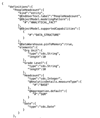
This is an excerpt of the JSON file that only shows the first Fact table. An in depth explanation of the JSON file is not part of this post. You can read the official documentation here. In general it is structured table by table and each table contains the column names as objects within “elements” with a datatype and - if applicable - a length and additional measure or dimension specific properties.
Uploading the JSON to Datasphere
After generating the JSON file on your local computer you need to upload it to Datasphere. Follow these steps.
Log in to your Datasphere tenant
- Navigate to the Data Builder and select New Entity - Relationship Model
In the empty ERM: Select Import → Import Objects from CSN/JSON File on the horizontal toolbar
Browse to the generated JSON file on your local machine
Click Next and select all files by clicking the checkbox on the top left (you can also specify to upload only single tables if that is what you want) → Click on Import CSN File
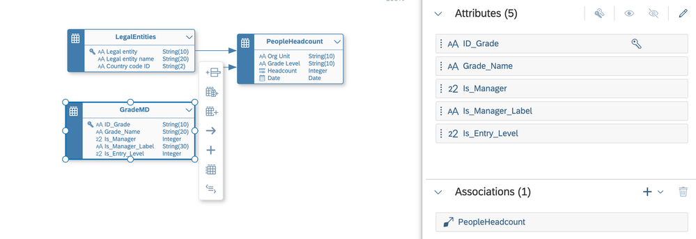
The Table structure is automatically generated. In this example the two Dimension tables are on the left and both are connected to the fact table to the right. The arrow direction shows that the association is defined in the dimension table, not in the fact table.
Datatypes, length, semantic usage types (fact and dimension), key-columns and associations are automatically detected.
Feel free to directly make changes / wrangle your data here by selecting a table. For example you should check if the measures and attributes in a fact table are correctly specified, since the python script can only assume whether a column is a measure or not.
After you made all your changes save (and optionally deploy) the model. Specify a name and location to save the model. After saving the ERM all tables are created.
You can now see the tables on the left Repository in the ERM Modeler or go back to data Builder and see them here:
If you directly deploy your model all tables within the model will be deployed.
Next steps
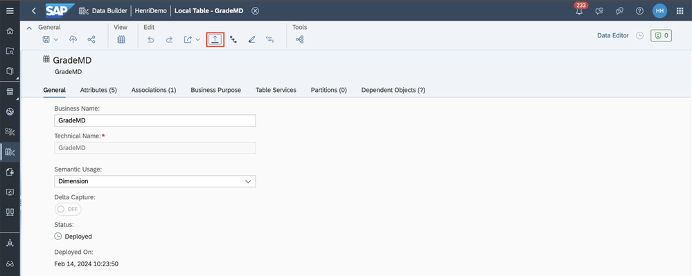
All of your dimension and fact tables, as well as their associations, are now in Datasphere. However, currently, only the table structures are present in Datasphere, without any data. To proceed, you can upload the data to your tables. Select the table and upload the CSV files to import data into the respective table.
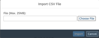
Click on choose file and select the CSV for this table from your local machine.
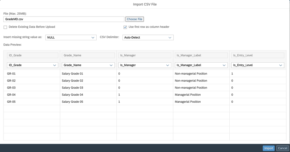
Keep the default settings when you first upload your data. Since we generated the table structure from the JSON the column names should be the same and are automatically mapped.
Next you can preview the uploaded data to validate if it has been uploaded correctly.
Repeat the upload process for every table.
After you uploaded the data to all tables you are fully prepared to build your views and models upon the uploaded tables. You can follow for example this tutorial from step 16 to create a consumable analytic model from your tables.
Conclusion
In Summary this blog post proposes a solution to automate the upload of various dimension and fact tables to SAP Datasphere. The script automatically detects tables, columns, semantic usages, keys, datatypes and associations. Once you run the script, it creates a JSON file that can be imported as an ERM to Datasphere. Saving the ERM creates the dimension and fact tables, so you can start uploading your data and building views and models right away!
Thanks for reading! For any questions or feedback feel free to leave a comment below the post.
- SAP Managed Tags:
- SAP Datasphere
You must be a registered user to add a comment. If you've already registered, sign in. Otherwise, register and sign in.
-
ABAP CDS Views - CDC (Change Data Capture)
2 -
AI
1 -
Analyze Workload Data
1 -
BTP
1 -
Business and IT Integration
2 -
Business application stu
1 -
Business Technology Platform
1 -
Business Trends
1,658 -
Business Trends
93 -
CAP
1 -
cf
1 -
Cloud Foundry
1 -
Confluent
1 -
Customer COE Basics and Fundamentals
1 -
Customer COE Latest and Greatest
3 -
Customer Data Browser app
1 -
Data Analysis Tool
1 -
data migration
1 -
data transfer
1 -
Datasphere
2 -
Event Information
1,400 -
Event Information
67 -
Expert
1 -
Expert Insights
177 -
Expert Insights
301 -
General
1 -
Google cloud
1 -
Google Next'24
1 -
GraphQL
1 -
Kafka
1 -
Life at SAP
780 -
Life at SAP
13 -
Migrate your Data App
1 -
MTA
1 -
Network Performance Analysis
1 -
NodeJS
1 -
PDF
1 -
POC
1 -
Product Updates
4,577 -
Product Updates
346 -
Replication Flow
1 -
REST API
1 -
RisewithSAP
1 -
SAP BTP
1 -
SAP BTP Cloud Foundry
1 -
SAP Cloud ALM
1 -
SAP Cloud Application Programming Model
1 -
SAP Datasphere
2 -
SAP S4HANA Cloud
1 -
SAP S4HANA Migration Cockpit
1 -
Technology Updates
6,873 -
Technology Updates
429 -
Workload Fluctuations
1
- Quick & Easy Datasphere - When to use Data Flow, Transformation Flow, SQL View? in Technology Blogs by Members
- Use CRUD Opreations with SAP Datasphere Command-Line-Interface in Technology Blogs by SAP
- SAP Build Process Automation Pre-built content for Finance Use cases in Technology Blogs by SAP
- CAP LLM Plugin – Empowering Developers for rapid Gen AI-CAP App Development in Technology Blogs by SAP
- Empowering Vendors: The Transformative Impact of SAP Chatbot in Technology Blogs by Members
| User | Count |
|---|---|
| 32 | |
| 17 | |
| 15 | |
| 14 | |
| 11 | |
| 9 | |
| 8 | |
| 8 | |
| 8 | |
| 7 |


