
- SAP Community
- Products and Technology
- Supply Chain Management
- SCM Blogs by Members
- Visual Basic (VBA) & SAP IBP (Integrated Business ...
Supply Chain Management Blogs by Members
Learn about SAP SCM software from firsthand experiences of community members. Share your own post and join the conversation about supply chain management.
Turn on suggestions
Auto-suggest helps you quickly narrow down your search results by suggesting possible matches as you type.
Showing results for
vincentverheyen
Active Participant
Options
- Subscribe to RSS Feed
- Mark as New
- Mark as Read
- Bookmark
- Subscribe
- Printer Friendly Page
- Report Inappropriate Content
02-13-2023
8:39 AM
Perhaps, in some of your own projects, your clients have expressed the request to be able to compare the absolute difference in value of a key figure between the Baseline and 1 or more Scenarios.
In the following tutorial, I will demonstrate how to do this, both for the total of the key figure, as well as for the key figure's value per Planning Object.
To do this, we will use a combination of the following:
- Totals
- Custom Excel formulas in Local Members
- Customized VBA Hookups (AFTER_REFRESH)
- Customized Visual Basic (VBA subroutines)
If you have never heard of, or combined Local Members, Visual Basic &/or VBA Hookups, hopefully the tutorial might be illuminating.
The SAP IBP Add-In for MS Excel provides multiple hooks (entry points for custom coding) to enhance functions of the Excel Add-In through MS Visual Basic for Applications (VBA) code.
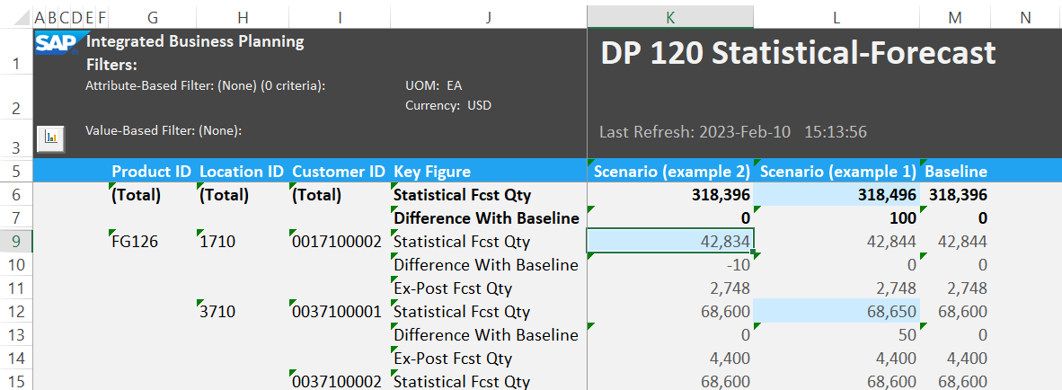
Let's start with a simple planning view "DP 120 Statistical Forecast" in Planning Area UNIPA. For simplicity, we will examine a planning view with 1 time bucket only (namely "Year: 2023"). Make sure to create 1 or more scenarios, to put the "Scenarios" in the Columns axis of your Planning View Layout, as such:

Planning View — DP 120 Statistical Forecast
Totals
To be able to show the totals of the key figure totals, we can take the following action (sum the total on the first attribute in the planning view):
"Edit View" > "Edit Planning View..." > "Attributes" > "Selected Attributes:" > "Product ID" > "Total Before":
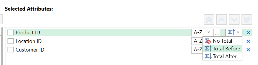
Selected Attributes — Product ID — Total Before
However, this will result in Totals on all key figures (in this case row 6 for key figure "Ex-Post Fcst Qty" and row 7 for key figure "Statistical Fcst Qty"):

Totals on all key figures
Totals on 1 key figure only (custom Visual Basic / VBA)
In case we only want to see the Totals on key figure "Statistical Fcst Qty", we could manually hide row 6. However, this will result in issues and bugs for the users later on, as they might switch the order of the key figures, add or hide more key figures, which will result in the wrong key figure being hidden.
Another way to hide the totals on the key figures we are not interested in (let's say we want to hide the Totals of "Ex-Post Fcst Qty"), would be to use the IBPFormattingSheet, perform "Add Member/Property" and:
- "Member Selection" > Key Figures" > "Ex-Post Fcst Qty" > "Add to Multiple Selection"
- & "Specific Selection" > Total Member
- & "Multiple Selection Overview" > Union
To then change the formatting in a way that the key figure values (Data) &/or the Header becomes invisible. For example by selecting the same text colour as the background colour of the cell.
However, this solution is also not completely satisfactory. Since, let's say the user wants the Totals (in our case key figure "Statistical Fcst Qty") to stay at the top of the planning view, even while scrolling down in the Planning View. This can be achieved by navigating, in the Planning View's sheet, to "View" > "Freeze Panes" > "Unfreeze Panes". Now click on cell K8, and "View" > "Freeze Panes" > "Freeze Panes".
The problem is namely, as you would now scroll down, even if you use the IBPFormattingSheet to make the text and values of "Ex-Post Fcst Qty" invisible, you will still lose a lot of vertical space (however many unnecessary rows, 1 per key figure of which the totals we are not interested in). And user's screens are only so large, so we would rather keep this vertical space for useful information.
Therefor, the only proper solution is to use custom VBA code, to be able to hide the unwanted key figures dynamically. It is possible to extend planning view workbooks with custom VBA implementations. You can add your custom VBA code directly into the planning view templates (or alternatively: call them from a separate custom .xlam Add-In).
For our purpose, we'll use and customize VBA hook AFTER_REFRESH. It is run after for example, after choosing Refresh, Save Data, Simulate in the SAP IBP ribbon in the Data Input section,or after changing planning view settings. For more information, see AFTER_REFRESH | SAP Help Portal.
To do this, select "Developer" > "Visual Basic". If there is no "Developer" section in your MS Excel Ribbon, a quick google will explain how to activate it.
Then navigate to "VBAProject (DP 120 Statistical Forecast.xlsm)" > "Modules" > "EpmAfterRefresh":

EpmAfterRefresh
If your template does not yet have this VBA Module, you can right-click on "Modules" > "Insert" > "Module", and rename the (Name) of the module to "EpmAfterRefresh". If you already have the module as shown in the screenshot above, then, before the line:
Ignore:... insert the following custom code:
'###################################################

'# SAP IBP & VBA: Hiding certain total key figures #

'# Vincent Verheyen                                #

'# SAP Community Blogs, 2023-02                    #

'###################################################

'# START OF CODE                                   #

'###################################################


Dim rFind As Range        'Variable to store the result of the search for "Key Figure"

Dim rCheck As Range        'Variable to store the range that needs to be checked for search terms

Dim rHide As Range        'Variable to store the row that needs to be hidden

Dim firstOccurrence As Boolean        'Variable to track if this is the first occurrence of the search term

Dim ws As Worksheet        'Variable to store the active worksheet

Dim searchTerms() As Variant        'Array to store the search terms

Dim lastRow As Long        'Variable to store the last row of the column containing "Key Figure"

Dim checkArray() As Variant        'Array to store the cells in the range being checked


searchTerms = Array("Ex-Post Fcst Qty")        'Setting the search terms to an array of strings. In this case we only look for the key figure "Ex-Post Fcst Qty".

Set ws = ThisWorkbook.ActiveSheet        'Setting the active worksheet to "ws"

Set rFind = ws.Range("5:5").Find(What:="Key Figure", LookIn:=xlValues)        'Finding the first cell in row 5 with the value "Key Figure"

lastRow = rFind.End(xlDown).Row        'Finding the last row in the column containing "Key Figure"

Set rCheck = rFind.Offset(1, 0).Resize(lastRow - 1, 1)        'Setting the range to be checked to the column containing "Key Figure", starting from the second row

rCheck.EntireRow.Hidden = False        'Unhiding all rows in the column containing "Key Figure"


If rFind.Offset(1, -1).Value = "(Total)" Then        'Checking if the cell one row below and one column to the left of the cell "Key Figure" is equal to "(Total)". In other words, this checks to see if there are "(Totals)" in the Planning View

checkArray = rCheck.Value        'Storing the values of the cells in the range being checked in an array

For i = LBound(searchTerms) To UBound(searchTerms)        'Looping through each search term

    firstOccurrence = True        'Setting firstOccurrence to True

    For j = 1 To UBound(checkArray, 1)        'Looping through each row in the array

        If InStr(1, checkArray(j, 1), searchTerms(i), vbTextCompare) > 0 Then        'Checking if the search term is present in the cell

        If firstOccurrence Then        'Checking if this is the first occurrence of the search term

        Set rHide = rCheck.Cells(j, 1)        'Setting rHide to the row of the cell containing the search term

        firstOccurrence = False        'Setting firstOccurrence to False

    Else

        Exit For        'Exiting the loop if this is not the first occurrence of the search term

    End If

End If

Next j

If Not rHide Is Nothing Then rHide.EntireRow.Hidden = True        'Hiding the row if a match was found

Next i

End If


'###################################################

'# END OF CODE                                     #

'###################################################

'# SAP IBP & VBA: Hiding certain total key figures #

'# Vincent Verheyen                                #

'# SAP Community Blogs, 2023-02                    #

'###################################################
Now when you click on "Refresh", only the Totals for key figure "Statistical Fcst Qty" will remain visible (= not hidden):

Totals on key figure Ex-Post Fcst Qty are now hidden
You can see that the custom VBA code has automatically hidden row 7 above, due to our customization of the VBA hook AFTER_REFRESH.
In cases where you want to hide several key figures, you just expand:
searchTerms = Array("Ex-Post Fcst Qty")into any list of key figures you want to hide, for example:
searchTerms = Array("Ex-Post Fcst Qty", "Recommended Safety Stock", "Sales Fcst Rev.")Compare Key Figure values in Baseline versus Scenarios (custom Excel formulas in Local Member)
Now, that we are able to customize which totals we want to show exactly. Let's look at how we can calculate and visualize the difference between the scenario and the baseline (remember "Compare Key Figure values in Baseline versus Scenarios" in the title of this article).
SAP does not have a standard method for this, so I went ahead and created my own custom Excel formula for this purpose.
Let's say we want to compare these key figure values for the key figure "Statistical Fcst Qty".
Click on "Template Admin" > "Report Editor" > "Local Member" and execute / enter the following:
- 1. Tick the checkbox "Enable" ✅
- 2. Name: DifferenceWithBaseline
- 3. Description: Difference With Baseline
- 4. Formula:
=EPMMEMBER([KEY_FIGURES].[].[STATISTICALFORECASTQTY])-INDIRECT(ADDRESS(ROW()-1,MATCH("Baseline",$A$5:$Z$5,0)))- 5. Tick the checkbox "Insert After" ✅
- 6. Under "Attached To", tick the checkbox "Member" ✅
- 7. Under "Attached To", at the right-hand side of the window click on the ellipsis (...) button, select "Key Figures", tick the checkbox "Statistical Fcst Qty" ✅ and click on OK
- 8. Under "Actions": click on Add at the bottom of the window
- 9. Finally, click on OK
If this does not change your planning view immediately, make sure you properly executed steps 1. and 8. above properly.
Let's explain the custom formula a bit.
- =EPMMEMBER([KEY_FIGURES].[].[STATISTICALFORECASTQTY]) returns the value of the key figure "Statistical Fcst Qty" from each Scenario (or in case of the column with "Baseline", from the Baseline)
- INDIRECT(ADDRESS(ROW()-1,MATCH("Baseline",$A$5:$Z$5,0))) returns the value of the same key figure, but only from the Baseline. IINDIRECT(ADDRESS(...)) will look for a row and a column number (to find the value we want to use). The column number is identified via the MATCH("Baseline",$A$5:$Z$5,0) which looks for an exact match of the text "Baseline" in the range $A$5:$Z$5 (= row 5) and returns the column number where the value "Baseline" is found. ROW()-1 returns the value of the row number of 1 row up from the current row in which this formula is used. Why do we choose 1 row up? Since, in steps 5., 6. and 7. above, we chose "Insert After", Attahed To "Member", "Key Figure:" "Statistical Fcst Qty".
- These two are substracted from eachother to create the difference.
If there might be any case in which you are unsure whether the text "Basline" will be in row 4, or in row 5, you could use a more complex formula:
=EPMMEMBER([KEY_FIGURES].[].[STATISTICALFORECASTQTY])-INDIRECT(ADDRESS(ROW()-1,IF(ISNA(MATCH("Baseline",$A$4:$Z$4,0)),MATCH("Baseline",$A$5:$Z$5,0),MATCH("Baseline",$A$4:$Z$4,0))))In this code the IF(...) function is used to conditionally determine the column number of the reference. If the text "Baseline" is not found as an exact match in row 4, it returns the column number using MATCH("Baseline",$A$5:$Z$5,0) (checking row 5). This not found in row 4' is checked using ISNA(...) to see if MATCH("Baseline",$A$4:$Z$4,0) (checking row 4) throws an #N/A error. If the value "Baseline" is found in the range $A$4:$Z$4 (checking row 4), then it simply returns the column number using MATCH("Baseline",$A$4:$Z$4,0) (= row 4).
When I was creating the formula above, I first took a much more (= much too) complicated approach, namely using a two-dimensional lookup by combining VLOOKUP(...) with MATCH(...). There I used many nested IF(...) statements to test all the possible columns in which the Totals of key figure "Statistical Fcst Quantity" might be found. For example, in the following complex formula we to try to find the text "Statistical Fcst Quantity" in column B (rows 6 to 12). If not found in column B, it looks in column C (rows 6 to 12), and so on until column M. If the text "Statistical Fcst Quantity" is found for example in column B, then the MATCH(...) function is used to find the position of the exact text match "Baseline" in the ranges B5:Z5 (row 5, columns B to Z). But if this was not the case, and if the text "Statistical Fcst Quantity" was found instead in column J for example, then the MATCH(...) function is used to find the position of the exact text match "Baseline" in the ranges J5:Z5 (row 5, columns J to Z), and so on.
=IFERROR(EPMMEMBER([KEY_FIGURES].[].[STATISTICALFORECASTQTY])-VLOOKUP("Statistical Fcst Qty",IF(NOT(ISNA(MATCH("Statistical Fcst Qty",B6:B12,0))),B6:Z12,IF(NOT(ISNA(MATCH("Statistical Fcst Qty",C6:C12,0))),C6:Z12,IF(NOT(ISNA(MATCH("Statistical Fcst Qty",D6:D12,0))),D6:Z12,IF(NOT(ISNA(MATCH("Statistical Fcst Qty",E6:E12,0))),E6:Z12,IF(NOT(ISNA(MATCH("Statistical Fcst Qty",F6:F12,0))),F6:Z12,IF(NOT(ISNA(MATCH("Statistical Fcst Qty",G6:G12,0))),G6:Z12,IF(NOT(ISNA(MATCH("Statistical Fcst Qty",H6:H12,0))),H6:Z12,IF(NOT(ISNA(MATCH("Statistical Fcst Qty",I6:I12,0))),I6:Z12,IF(NOT(ISNA(MATCH("Statistical Fcst Qty",J6:J12,0))),J6:Z12,IF(NOT(ISNA(MATCH("Statistical Fcst Qty",K6:K12,0))),K6:Z12,IF(NOT(ISNA(MATCH("Statistical Fcst Qty",L6:L12,0))),L6:Z12,M6:Z12))))))))))),MATCH("Baseline",IF(NOT(ISNA(MATCH("Statistical Fcst Qty",B6:B12,0))),B5:Z5,IF(NOT(ISNA(MATCH("Statistical Fcst Qty",C6:C12,0))),C5:Z5,IF(NOT(ISNA(MATCH("Statistical Fcst Qty",D6:D12,0))),D5:Z5,IF(NOT(ISNA(MATCH("Statistical Fcst Qty",E6:E12,0))),E5:Z5,IF(NOT(ISNA(MATCH("Statistical Fcst Qty",F6:F12,0))),F5:Z5,IF(NOT(ISNA(MATCH("Statistical Fcst Qty",G6:G12,0))),G5:Z5,IF(NOT(ISNA(MATCH("Statistical Fcst Qty",H6:H12,0))),H5:Z5,IF(NOT(ISNA(MATCH("Statistical Fcst Qty",I6:I12,0))),I5:Z5,IF(NOT(ISNA(MATCH("Statistical Fcst Qty",J6:J12,0))),J5:Z5,IF(NOT(ISNA(MATCH("Statistical Fcst Qty",K6:K12,0))),K5:Z5,IF(NOT(ISNA(MATCH("Statistical Fcst Qty",L6:L12,0))),L5:Z5,M5:Z5))))))))))),0),FALSE),"Revert to original template.")So in short, this advanced formula looks for the exact match of "Statistical Fcst Quantity" to identify the row of the value to look-up (between rows 6 and 12), and we used the nested IF(...) statements to test all the possible columns (B to M) in which "Statistical Fcst Quantity" could be found; while the column to look-up was identified by looking for the exact match of "Baseline" in row 5 (between the column identified, to Z). The IFERROR(...) function is used returns the string "Revert to original template.", for example in the case that these exact matches never occurred in the range B6 to Z12.
The reason that this formula is so complex, is because there is a limitation on VLOOKUP(...), which you'll equally encounter when trying to substitute it with INDEX(...) and XLOOKUP(...). See for example the Microsoft Excel documentation VLOOKUP function - Microsoft Support:
"Remember that the lookup value should always be in the first column in the range for VLOOKUP to work correctly. For example, if your lookup value is in cell C2 then your range should start with C."
You can test this formula and see that it also works, for the totals, if they are within B6 to Z12. Why did I choose rows 6 to 12? Because we were working in a certain Planning View with 6 different Key Figures which were by default in that Planning View. So, even if they changed the order of the Key Figures, the code would still retrieve the correct row. However, this code is not practical for large ranges, and will also start to create incorrect calculations in the non-total rows.
Therefor, once I realized we could much better use INDIRECT(ADDRESS(ROW()-1, the formula became so much simpler. So for most purposes I would advise you to use the simple formula from step 4. above, namely:
=EPMMEMBER([KEY_FIGURES].[].[STATISTICALFORECASTQTY])-INDIRECT(ADDRESS(ROW()-1,MATCH("Baseline",$A$5:$Z$5,0)))This should create the following result (you can slightly modify the numbers in the Scenario, to see that this indeed yields the correct calculation):
Calculate the Difference with Baseline (in Local Member) for key figure Statistical Fcst Qty
Also if we add an extra Scenario, you can see, the calculations are still correct:
Difference with Baseline, still works for multiple Scenarios
Note that this generates the Difference With Baseline for each Planning Object, not only for the Totals (Total) at the top.
... with custom formatting for easy searchability (IBPFormattingSheet & CTRL-F)
You could use custom formatting in the IBPFormattingSheet, to make the positive or negative differences more visible. For example, we might want to achieve the following:
- Positive differences (when the Scenario's Key Figure value is higher than the Baseline) should receive a red flag 🚩
- Negative differences (when the Scenario's Key Figure value is lower than the Baseline) should receive a green arrow ▼
- If there is no difference, show the grey text "equal Stat. Fcst Qty" instead of 0.
This can be achieved via "Edit View > "View Formats", and then click on the sheet "IBPFormattingSheet" (a faster way is to just right-click on the current sheet tab, and select "Unhide" > "IBPFormattingSheet").
Via the following custom formatting:
In column B, find the grey area which says "Row" > at the bottom, click on "Add Member/Property" > "Add Condition" > "Specific Selection" > tick the checkbox "Local Member" ✅ > next to the field "Name of the local member:", write "DifferenceWithBaseline" > click "OK" > click "OK"
Now, in the newly created row, which says "DifferenceWithBaseline" in column C, go to that row's cell in column F (the column says "Data" at the top), and right-click on that cell (the standard value in that cell would be "1000"). After right-clicking, choose "Format Cells..." > "Number" tab > "Custom".
Under "Type:" by default is written "General". Change this into the following formula:
[Color16][=0]"equal Stat. Fcst Qty";[Red][>0]"+"#,##0.00 "unit(s) 🚩";[Color10]#,##0.00 "unit(s) ▼"I will try to make the code a bit more readable by applying the effect of the ColorIndex colors in the code:
- [Color16][=0]"equal Stat. Fcst Qty";[Red][>0]"+"#,##0.00 "unit(s) 🚩";[Color10]#,##0.00 "unit(s) ▼"
This will yield the following result:

Difference with Baseline, with customized number formatting in IBPFormattingSheet
I'll show you 1 more trick as to why this can be extremely handy for the end-users. Because an end-user can now simply control-find:
"CTRL-F" > Find What: "+" > click on: "Find All"
This will make the user get a complete list of all the Positive Differences With Baseline (i.e. all the cell's which contain a "+" character).

Easy scrolling through all positive (+) values using CTRL-F
Note that in the screenshot, in the list in the "Find and Replace" window we have clicked on the second row (highlighted in dark blue), which immediately scrolls in our Planning View to the correct cell (L13), and highlights it by auto-clicking. If you have a long list, you can simply click "Find Next", which allows the planner to scroll to the values that need their attention, throughout the Planning View.
For the negative values, in case CTRL-F on the minus symbol "-" would yield unwanted results, one could CTRL-F directly on the custom character or text instead, such as "▼".
If you click on "Value" inside the CTRL-F table, you will even find that your values are sorted from large to small! Even easier for the end-users to priotise important differences.
Only compare Key Figure values in Baseline versus Scenarios for Totals only, with the click of a button (custom VBA subroutine)
To showcase one more possibility in customizing Planning Views using Visual Basic, let's introduce a button by which we are able to ONLY show the Differences for the Totals, instead of the Differences for each Planning Object, as was the case above.
Click "Insert" > "Illustrations" > "Shapes"
Choose any Shape, and type some text in it. In our case we'll add the text "Toggle "Difference With Baseline" on individual Planning Objects (≠ Total)" inside the purple button:

Button to run custom VBA code
We can put our custom VBA code, for example in a new Module. To do this, navigate to "Developer" > "VBAProject (DP 120 Statistical Forecast.xlsm)" > right-click on "Modules" > "Insert" > "Module", and rename the (Name) of the module to for example "HideDiff".
'###################################################

'# SAP IBP & VBA: Button to toggle non-total KFs   #

'# Vincent Verheyen                                #

'# SAP Community Blogs, 2023-02                    #

'###################################################

'# START OF CODE                                   #

'###################################################


Sub HideDiff()


Application.ScreenUpdating = False        'disable screen updates to improve performance while rows are being hidden or unhidden


Dim rFind As Range        'Range to store the location of the keyword "Key Figure"

Dim rCheck As Range        'Range to store the cells to check for the keyword "Difference With Baseline"

Dim ws As Worksheet        'Worksheet object to store the active worksheet

Dim lastRow As Long        'Variable to store the last row of the data

Dim arrCheck As Variant        'Array to store the cells to check for the keyword "Difference With Baseline"

Dim firstOccurrence As Boolean        'Boolean to keep track of first occurrence of "Difference With Baseline"

Dim i As Long        'Variable to keep track of the loop


Set ws = ThisWorkbook.ActiveSheet        'Set the worksheet object to the active worksheet

Set rFind = ws.Range("5:5").Find(What:="Key Figure", LookIn:=xlValues)        'Find the location of the keyword "Key Figure"

lastRow = rFind.End(xlDown).Row        'Determine the last row of the data

Set rCheck = rFind.Offset(1, 0).Resize(lastRow, 1)        'Set the range of cells to check for the keyword "Difference With Baseline"

arrCheck = rCheck.Value        'Copy the range into an array

firstOccurrence = True        'Set the first occurrence Boolean to True


If rFind.Offset(1, -1).Value = "(Total)" Then        'Check if the cell to the left of the keyword "Key Figure" is equal to "(Total)"

For i = 1 To UBound(arrCheck, 1)        'Loop through the array of cells to check

    If InStr(1, arrCheck(i, 1), "Difference With Baseline", vbTextCompare) > 0 Then        'Check if the cell contains the keyword "Difference With Baseline"

    If firstOccurrence Then        'Check if this is the first occurrence of the keyword

    firstOccurrence = False        'Set the first occurrence Boolean to False

Else

    If rCheck(i, 1).EntireRow.Hidden = True Then        'Check if the row is currently hidden

    rCheck(i, 1).EntireRow.Hidden = False        'Unhide the row

Else

    rCheck(i, 1).EntireRow.Hidden = True        'Hide the row

End If

End If

End If

Next i


Else

    For i = 1 To UBound(arrCheck, 1)        'Loop through the array of cells to check

        If InStr(1, arrCheck(i, 1), "Difference With Baseline", vbTextCompare) > 0 Then        'Check if the cell contains the keyword "Difference With Baseline"

        If rCheck(i, 1).EntireRow.Hidden = True Then        'Check if the row is currently hidden

        rCheck(i, 1).EntireRow.Hidden = False        'Unhide the row

    Else

        rCheck(i, 1).EntireRow.Hidden = True        'Hide the row

    End If

End If

Next i


End If


Application.ScreenUpdating = True        're-enable screen updates


End Sub


'###################################################

'# SAP IBP & VBA: Button to toggle non-total KFs   #

'# Vincent Verheyen                                #

'# SAP Community Blogs, 2023-02                    #

'###################################################

'# END OF CODE                                     #

'###################################################
Now go back to your purple button, and right-click on it and choose "Assign Macro..." and select "'DP 120 Statistical Forecast.xlsm'!HideDiff.HideDiff", and click "OK".
If you click the button once, the result will hide all of the rows "Difference With Baseline", and only keep the occurence of "Difference With Baseline" which occurs:

Difference With Baseline per Planning Object will be hidden after clicking the button
If you click the button again, the result will show the rows once again, for each Planning Object:
Difference With Baseline per Planning Object will be shown after clicking the button again
So we have created a button via which you can easily toggle the hiding or showing of rows.
Freeze Panes
Now that we have finalized the Planning View, as a finishing touch, let's freeze the panes, such that the Totals (and the Differences) always stay visible, when scrolling. In the Planning View’s sheet, navigate to “View” > “Freeze Panes” > “Unfreeze Panes”. Now click on cell K9, and “View” > “Freeze Panes” > “Freeze Panes”.
Welcome to get in touch
Did you find this example of VBA customization of SAP IBP helpful? If so, feel free to leave a comment, like, follow, or simply get in touch!
- SAP Managed Tags:
- SAP Integrated Business Planning for Supply Chain,
- EPM Add-In for Excel
4 Comments
You must be a registered user to add a comment. If you've already registered, sign in. Otherwise, register and sign in.
Labels in this area
-
aATP
1 -
ABAP Programming
1 -
Activate Credit Management Basic Steps
1 -
Adverse media monitoring
1 -
Alerts
1 -
Ausnahmehandling
1 -
bank statements
1 -
Bin Sorting sequence deletion
1 -
Bin Sorting upload
1 -
BP NUMBER RANGE
1 -
Brazil
1 -
Business partner creation failed for organizational unit
1 -
Business Technology Platform
1 -
Central Purchasing
1 -
Change History
1 -
Charge Calculation
2 -
Cloud Extensibility
1 -
Compliance
1 -
Controlling
1 -
Controlling Area
1 -
Data Enrichment
1 -
DIGITAL MANUFACTURING
1 -
digital transformation
1 -
Dimensional Weight
1 -
Direct Outbound Delivery
1 -
E-Mail
1 -
ETA
1 -
EWM
6 -
EWM - Delivery Processing
2 -
EWM - Goods Movement
4 -
EWM Monitor
1 -
EWM Outbound configuration
1 -
EWM-RF
1 -
EWM-TM-Integration
1 -
Extended Warehouse Management (EWM)
3 -
Extended Warehouse Management(EWM)
7 -
Finance
1 -
Freight Settlement
1 -
FUB_Strategy
1 -
FUBR
1 -
Geo-coordinates
1 -
Geo-routing
1 -
Geocoding
1 -
Geographic Information System
1 -
GIS
1 -
Goods Issue
2 -
GTT
2 -
IBP inventory optimization
1 -
inbound delivery printing
1 -
Incoterm
1 -
Innovation
1 -
Inspection lot
1 -
intraday
1 -
Introduction
1 -
Inventory Management
1 -
Localization
1 -
Logistics Optimization
1 -
Map Integration
1 -
Material Management
1 -
Material Master changes
1 -
Materials Management
1 -
MFS
1 -
New Feature
1 -
Outbound with LOSC and POSC
1 -
Packaging
1 -
PPF
1 -
PPOCE
1 -
PPOME
1 -
print profile
1 -
Process Controllers
1 -
Production process
1 -
QM
1 -
QM in procurement
1 -
Real-time Geopositioning
1 -
Risk management
1 -
S4 HANA
1 -
S4 HANA 2022
1 -
S4-FSCM-Custom Credit Check Rule and Custom Credit Check Step
1 -
S4SCSD
1 -
Sales and Distribution
1 -
SAP DMC
1 -
SAP ERP
1 -
SAP Extended Warehouse Management
2 -
SAP Hana Spatial Services
1 -
SAP IBP IO
1 -
SAP MM
1 -
sap production planning
1 -
SAP QM
1 -
SAP REM
1 -
SAP repetiative
1 -
SAP S4HANA
1 -
SAP TM
1 -
SAP Transportation Management
3 -
SAP Variant configuration (LO-VC)
1 -
SAPTM
1 -
SD (Sales and Distribution)
1 -
Shotcut_Scenario
1 -
Source inspection
1 -
Storage bin Capacity
1 -
Supply Chain
1 -
Supply Chain Disruption
1 -
Supply Chain for Secondary Distribution
1 -
Technology Updates
1 -
TMS
1 -
Transportation Cockpit
1 -
Transportation Management
2 -
Visibility
2 -
warehouse door
1 -
WOCR
1
- « Previous
- Next »
Related Content
- Enhanced Shortcut Scenario SAP TM in Supply Chain Management Blogs by Members
- SAP Business Network for Logistics 2404 Release – What’s New? in Supply Chain Management Blogs by SAP
- SAP IBP Real-Time Integration: Empowering Businesses for Smarter, Faster Decisions in Supply Chain Management Blogs by SAP
- AI-powered supply chain solutions: Better decisions, better outcomes in Supply Chain Management Blogs by SAP
- What's new with Collaborative Maintenance? in Supply Chain Management Blogs by SAP
Top kudoed authors
| User | Count |
|---|---|
| 9 | |
| 5 | |
| 4 | |
| 3 | |
| 1 | |
| 1 | |
| 1 | |
| 1 | |
| 1 | |
| 1 |