

- SAP Community
- Products and Technology
- Technology
- Technology Blogs by SAP
- Running Year to Date (YTD) on fiscal periods with ...
Technology Blogs by SAP
Learn how to extend and personalize SAP applications. Follow the SAP technology blog for insights into SAP BTP, ABAP, SAP Analytics Cloud, SAP HANA, and more.
Turn on suggestions
Auto-suggest helps you quickly narrow down your search results by suggesting possible matches as you type.
Showing results for
Product and Topic Expert
Options
- Subscribe to RSS Feed
- Mark as New
- Mark as Read
- Bookmark
- Subscribe
- Printer Friendly Page
- Report Inappropriate Content
11-01-2023
4:34 PM
In this blog post we'll take you through the options to model a running Year to Date (YTD) metric in SAP Datasphere, using different approaches. This blog post is the third of the following series:
Let's go over a few reasons to model a YTD metric in SAP Datasphere as described in this blog:
The YTD calculation in this blog is based on fiscal periods, but you can also base the calculation on other time characteristics, fiscal or not, such as calendar week, calendar month or fiscal quarter.
We start with a sample set of transactions. The data set consists of 25+ million records, so that we can also say something about performance of the different views and queries. First we join the transaction table with the fiscal calendar of the previous blog post. It's a simple inner join of the transaction date with the date of the fiscal calendar. Now we have the fiscal year and fiscal period as par of our transaction data, which are the base attributes for our YTD metrics.
Skip to the next section if you're looking for a running YTD result. But if you just want a single YTD value of a specific year and period as a result, this would be achieved by using a simple filter. For example, you could use a restricted measure filter in an Analytic Model, which will prompt a user to select a certain fiscal period. You would first define the restricted measure variable as depicted below.
After defining the restricted measure, you apply the variable filter inside a restricted measure, as depicted below.
In below data preview of the Analytic Model editor, I chose period 6 when prompted for the variable, which yields the result as depicted below.
Ok, that was pretty simple, as it's just a sum with a filter applied. You can model this in a SQL View, in a Graphical View, or in an Analytic View as shown above. But what if we want to show running (aka cumulative) YTD figures, where for each period a YTD value sums up the previous periods?
To get to a running YTD result, where each period is displayed with its running YTD value, we have to turn to SQL. Broadly speaking, there are two main options. One uses a window function, and the other uses a join with a helper table. In this section we explain the window function option and in the next section the join with a helper table. In SAP Datasphere, we write the SQL inside a SQL View defined with semantic usage "fact", so that we can use the view subsequently in an Analytic Model.
With a window function you can write quite an elegant SQL statement. An example SQL statement is pasted below. There are two main parts to the query:
In case you're not familiar with window functions, let's explain what the window function does in this case. Each resulting row from the subquery represents a fiscal period. For each row, the window function works with a partition window. In this case, the window contains all rows having the same year that the current row is in, from the first row of the partition up until the current row. Why up until the current row you may ask? Well, that's default partition window behavior, and the default is exactly what we need. As the rows are ordered by period, the partition window contains the current and previous periods. And these are summed up into the YTD amount.
So the basics are actually pretty simple, once you get how window functions work. It becomes a bit more complex when you have more advanced requirements than just displaying the YTD values per period. What if you have to slice the result by additional attributes? In that case, you will have to take such attribute up in your query. As an example, see below how the query is adjusted to report YTD values per product, in addition to year and period.
As you can see, you need to adjust the entire query to account for slicing the result on another attribute. And you have to be a bit careful here as well: by adding attributes, you are increasing the result set of the subquery. That's fine if the subquery result set remains rather small. If that subset becomes rather large, the window function will take its toll. Even if you slice out the attribute in a downstream view or tool, summarizing the result of the query again, the subquery that the window function operates on will not get smaller.
Also, be aware that there is a limitation to the use of window functions for this use case, namely that the subquery that you are using has to have data for each period in the past. If not, the period for which there is no data, will not be part of the result at all. For productive use cases, this will likely not happen when your subquery aggregates on the rather high level of year and period. But in case you would extend the query, or filter the query, let's say by attribute "product", a product might have periods for which there is no data. This might be acceptable when it only looks a bit weird: you won't see the periods displayed for which there were no values. But be careful when using that query result in another query or tool; when you would take out the "product" dimension to roll up to just year and period, the YTD sums are not correct.
A classical method to create a running YTD result using SQL, is with a helper table. Again there are multiple options, and here I use the simplest helper table I could think of. We define a helper table with simply an enumeration of the periods in a year, in my case 12. For this, we create a local table with one column, and use the Table Editor function to enter the different values, as you can see below.
The period list helper table will enable summing up previous periods in a fiscal year by a non-equi join of the transaction data period with the period list. See the SQL statement and result set below. The SQL query consists of the following parts:
You can see that the result is the same as with the window function. Only the way to calculate it is different. There is a benefit though with this approach: even if your subquery result has gaps, meaning that for certain periods there are no actuals, the YTD values are still calculated and displayed. In case you extend the query with other attributes, and afterwards roll-up that query again, the result will still be correct. Still take into account though that with a large result set of the subquery, the join with the helper table and the CASE logic will take its toll, just like with the window function option. In my tests, the window function option proved to be slightly more performant.
The above query uses a non-equi join and a straighforward table with an enumeration of periods to make the roll up. However, we could also use a somewhat more advanced period table or view, so that we can use an equi-join, which some people argue is more performant than a non-equi join. If your subquery is small, it all doesn't matter, but if your subquery is larger, it might. However, in my own tests on a 25mio+ data set and 20mio subquery result, the non-equi join actually performed better.
But if you insist, in order to do this, you could define a table with two columns: F_PERIOD and F_PERIOD_MAPPED, and fill it as the following data preview shows. For each period, you map to each period to be rolled up.
The query would look slightly different, as shown in below code snippet.
But again, in my tests, this query performed worse than the non-equi join. Approximately, the query ran about twice as long.
The SQL definitions can be written inside a SQL View, which in SAP Datasphere you would probably define with semantic usage "fact". This way, you can directly consume the SQL view in your Analytic Model. Taking one of the queries defined above, it would look as follows.
The YTD logic is defined in your SQL view, and with that, your Analytic Model might look quite simple. You can of course define additional filters, but then make sure you push those down to the subquery of the SQL View. And maybe you have added a few attributes to the SQL result set, and for those attributes you could associate dimensions. This should all be fine, as long as you take into account that the result set does not become too large and therefore expensive.
This blog presented two main options to write logic for a running YTD result: one with a window function and one with a helper table. When deciding for which option, take the following factors into account:
In a subsequent blog, I'll dive into other metrics, such as a rolling 12-month average or period-on-period comparisons.
- Fiscal calendar generation for SAP Datasphere using built-in procedure
- Standalone and week-based fiscal calendar generation for SAP Datasphere
- Running Year to Date (YTD) on fiscal periods with SAP Datasphere (this post)
Let's go over a few reasons to model a YTD metric in SAP Datasphere as described in this blog:
- SAP Datasphere, at time of writing, does not include ready-to-go OLAP features to define YTD metrics or other types of running totals;
- SAP Analytics Cloud offers YTD and other running or rolling time metrics out of the box, but (again at time of writing) does not support it for fiscal calendars on SAP Datasphere. Also for Gregorian calendar-based data, there are some limitations;
- You have another (front-end) tool that connects to SAP Datasphere which might not support such time-based metrics at all;
- You want to centrally define such metrics.
The YTD calculation in this blog is based on fiscal periods, but you can also base the calculation on other time characteristics, fiscal or not, such as calendar week, calendar month or fiscal quarter.
Join transaction data with fiscal calendar
We start with a sample set of transactions. The data set consists of 25+ million records, so that we can also say something about performance of the different views and queries. First we join the transaction table with the fiscal calendar of the previous blog post. It's a simple inner join of the transaction date with the date of the fiscal calendar. Now we have the fiscal year and fiscal period as par of our transaction data, which are the base attributes for our YTD metrics.

Figure 1: Fact view with a join between transaction date and fiscal calendar date
Simply getting a YTD value (we're not running yet)
Skip to the next section if you're looking for a running YTD result. But if you just want a single YTD value of a specific year and period as a result, this would be achieved by using a simple filter. For example, you could use a restricted measure filter in an Analytic Model, which will prompt a user to select a certain fiscal period. You would first define the restricted measure variable as depicted below.

Figure 2: Restricted measure definition in an analytic model
After defining the restricted measure, you apply the variable filter inside a restricted measure, as depicted below.

Figure 3: Apply variable in a restricted measure
In below data preview of the Analytic Model editor, I chose period 6 when prompted for the variable, which yields the result as depicted below.

Figure 4: Result in the analytic modeler when filtering on period == 6
Ok, that was pretty simple, as it's just a sum with a filter applied. You can model this in a SQL View, in a Graphical View, or in an Analytic View as shown above. But what if we want to show running (aka cumulative) YTD figures, where for each period a YTD value sums up the previous periods?
Running YTD - option 1 - window function
To get to a running YTD result, where each period is displayed with its running YTD value, we have to turn to SQL. Broadly speaking, there are two main options. One uses a window function, and the other uses a join with a helper table. In this section we explain the window function option and in the next section the join with a helper table. In SAP Datasphere, we write the SQL inside a SQL View defined with semantic usage "fact", so that we can use the view subsequently in an Analytic Model.
With a window function you can write quite an elegant SQL statement. An example SQL statement is pasted below. There are two main parts to the query:
- A subquery that sums up the amount by year and period;
- A select on the subquery, of which YTD_AMOUNT defines the rolling YTD behavior using a window function.
In case you're not familiar with window functions, let's explain what the window function does in this case. Each resulting row from the subquery represents a fiscal period. For each row, the window function works with a partition window. In this case, the window contains all rows having the same year that the current row is in, from the first row of the partition up until the current row. Why up until the current row you may ask? Well, that's default partition window behavior, and the default is exactly what we need. As the rows are ordered by period, the partition window contains the current and previous periods. And these are summed up into the YTD amount.
--YTD window function with subquery

SELECT

  F_YEAR,

  F_PERIOD,

  PERIOD_AMOUNT,

  SUM(PERIOD_AMOUNT) OVER (PARTITION BY F_YEAR ORDER BY F_PERIOD)

    AS YTD_AMOUNT

FROM (

  SELECT

    F_YEAR,

    F_PERIOD,

    SUM(AMOUNT) AS PERIOD_AMOUNT

  FROM

    FT_TX_FISCPER

  GROUP BY

    F_YEAR, F_PERIOD

)

ORDER BY

  F_YEAR, F_PERIOD;
Figure 5: Result of the YTD query with window function
So the basics are actually pretty simple, once you get how window functions work. It becomes a bit more complex when you have more advanced requirements than just displaying the YTD values per period. What if you have to slice the result by additional attributes? In that case, you will have to take such attribute up in your query. As an example, see below how the query is adjusted to report YTD values per product, in addition to year and period.
--YTD, now based on product

SELECT

  PRODUCT,

  F_YEAR,

  F_PERIOD,

  PERIOD_AMOUNT,

  SUM(PERIOD_AMOUNT) OVER (PARTITION BY PRODUCT, F_YEAR ORDER BY F_PERIOD) AS YTD_AMOUNT

FROM (

  SELECT

    PRODUCT,

    F_YEAR,

    F_PERIOD,

    SUM(AMOUNT) AS PERIOD_AMOUNT

  FROM

    FT_TX_FISCPER

  GROUP BY

    PRODUCT, F_YEAR, F_PERIOD

)

ORDER BY

  PRODUCT, F_YEAR, F_PERIOD;
As you can see, you need to adjust the entire query to account for slicing the result on another attribute. And you have to be a bit careful here as well: by adding attributes, you are increasing the result set of the subquery. That's fine if the subquery result set remains rather small. If that subset becomes rather large, the window function will take its toll. Even if you slice out the attribute in a downstream view or tool, summarizing the result of the query again, the subquery that the window function operates on will not get smaller.
Also, be aware that there is a limitation to the use of window functions for this use case, namely that the subquery that you are using has to have data for each period in the past. If not, the period for which there is no data, will not be part of the result at all. For productive use cases, this will likely not happen when your subquery aggregates on the rather high level of year and period. But in case you would extend the query, or filter the query, let's say by attribute "product", a product might have periods for which there is no data. This might be acceptable when it only looks a bit weird: you won't see the periods displayed for which there were no values. But be careful when using that query result in another query or tool; when you would take out the "product" dimension to roll up to just year and period, the YTD sums are not correct.
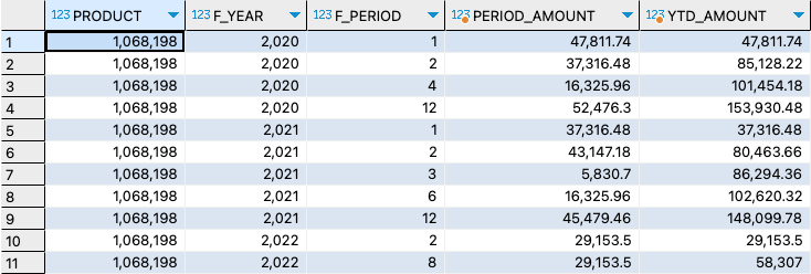
Figure 6: Gaps in YTD result if not all periods have data for a product
Running YTD - option 2 - join with helper table
A classical method to create a running YTD result using SQL, is with a helper table. Again there are multiple options, and here I use the simplest helper table I could think of. We define a helper table with simply an enumeration of the periods in a year, in my case 12. For this, we create a local table with one column, and use the Table Editor function to enter the different values, as you can see below.

Figure 7: Local table with a list of periods in a fiscal year
The period list helper table will enable summing up previous periods in a fiscal year by a non-equi join of the transaction data period with the period list. See the SQL statement and result set below. The SQL query consists of the following parts:
- A subquery that sums up the amount by year and period;
- A non-equi join which joins each period with all subsequent periods of the fiscal year;
- The F_PERIOD_AMOUNT column sums only the amount for current period, using a CASE statement;
- The YTD_AMOUNT column sums up all rows, and with that, represents the running YTD values.
--YTD using period list and subquery

SELECT

  F_YEAR,

  P.F_PERIOD,

  SUM(CASE WHEN T.F_PERIOD = P.F_PERIOD THEN PERIOD_AMOUNT ELSE 0 END)

    AS F_PERIOD_AMOUNT,

  SUM(PERIOD_AMOUNT) AS YTD_AMOUNT

FROM (

  SELECT

    F_YEAR,

    F_PERIOD,

    SUM(AMOUNT) AS PERIOD_AMOUNT

  FROM

    FT_TX_FISCPER

  GROUP BY

    F_YEAR, F_PERIOD

) T

JOIN

  LT_PERIODLIST P ON T.F_PERIOD <= P.F_PERIOD

GROUP BY

  F_YEAR, P.F_PERIOD

ORDER BY

  F_YEAR, P.F_PERIOD;
Figure 8: Output of the YTD query with helper table
You can see that the result is the same as with the window function. Only the way to calculate it is different. There is a benefit though with this approach: even if your subquery result has gaps, meaning that for certain periods there are no actuals, the YTD values are still calculated and displayed. In case you extend the query with other attributes, and afterwards roll-up that query again, the result will still be correct. Still take into account though that with a large result set of the subquery, the join with the helper table and the CASE logic will take its toll, just like with the window function option. In my tests, the window function option proved to be slightly more performant.
Performance of equi join versus non-equi join
The above query uses a non-equi join and a straighforward table with an enumeration of periods to make the roll up. However, we could also use a somewhat more advanced period table or view, so that we can use an equi-join, which some people argue is more performant than a non-equi join. If your subquery is small, it all doesn't matter, but if your subquery is larger, it might. However, in my own tests on a 25mio+ data set and 20mio subquery result, the non-equi join actually performed better.
But if you insist, in order to do this, you could define a table with two columns: F_PERIOD and F_PERIOD_MAPPED, and fill it as the following data preview shows. For each period, you map to each period to be rolled up.

Figure 9: Period mapping table
The query would look slightly different, as shown in below code snippet.
--YTD using period mapping helper table

SELECT

  F_YEAR,

  P.F_PERIOD,

  SUM(CASE WHEN T.F_PERIOD = P.F_PERIOD THEN AMOUNT ELSE 0 END)

    AS F_PERIOD_AMOUNT,

  SUM(AMOUNT) AS YTD_AMOUNT

FROM

  FT_TX_FISCPER T

INNER JOIN

 LV_YTD_PERIOD_MAPPING P ON T.F_PERIOD = P.F_PERIOD_MAPPED

GROUP BY

  F_YEAR, P.F_PERIOD

ORDER BY

  F_YEAR, P.F_PERIOD;
But again, in my tests, this query performed worse than the non-equi join. Approximately, the query ran about twice as long.
How to get from SQL to an Analytic Model?
The SQL definitions can be written inside a SQL View, which in SAP Datasphere you would probably define with semantic usage "fact". This way, you can directly consume the SQL view in your Analytic Model. Taking one of the queries defined above, it would look as follows.

Figure 10: For sake of completeness, a screenshot of a SQL View inside SAP Datasphere
The YTD logic is defined in your SQL view, and with that, your Analytic Model might look quite simple. You can of course define additional filters, but then make sure you push those down to the subquery of the SQL View. And maybe you have added a few attributes to the SQL result set, and for those attributes you could associate dimensions. This should all be fine, as long as you take into account that the result set does not become too large and therefore expensive.
Conclusion
This blog presented two main options to write logic for a running YTD result: one with a window function and one with a helper table. When deciding for which option, take the following factors into account:
- Clarity of SQL: window functions just needs a single line, no joins;
- Speed of development: window functions don't need a helper table, which does not need to be maintained and ingested with data (in dev, test, prod, etc.);
- Performance: similar as long as the running total is calculated on a small set of data, like a subquery with only year and period. If the subquery result set becomes larger, you might start to see differences, but you'll have to test yourself to see what works better. In my case the window function was a bit faster;
- Correct result: go for the helper table if you expect gaps in your data.
In a subsequent blog, I'll dive into other metrics, such as a rolling 12-month average or period-on-period comparisons.
- SAP Managed Tags:
- SAP Datasphere,
- SAP HANA Cloud,
- SQL
Labels:
3 Comments
You must be a registered user to add a comment. If you've already registered, sign in. Otherwise, register and sign in.
Labels in this area
-
ABAP CDS Views - CDC (Change Data Capture)
2 -
AI
1 -
Analyze Workload Data
1 -
BTP
1 -
Business and IT Integration
2 -
Business application stu
1 -
Business Technology Platform
1 -
Business Trends
1,658 -
Business Trends
93 -
CAP
1 -
cf
1 -
Cloud Foundry
1 -
Confluent
1 -
Customer COE Basics and Fundamentals
1 -
Customer COE Latest and Greatest
3 -
Customer Data Browser app
1 -
Data Analysis Tool
1 -
data migration
1 -
data transfer
1 -
Datasphere
2 -
Event Information
1,400 -
Event Information
67 -
Expert
1 -
Expert Insights
177 -
Expert Insights
301 -
General
1 -
Google cloud
1 -
Google Next'24
1 -
GraphQL
1 -
Kafka
1 -
Life at SAP
780 -
Life at SAP
13 -
Migrate your Data App
1 -
MTA
1 -
Network Performance Analysis
1 -
NodeJS
1 -
PDF
1 -
POC
1 -
Product Updates
4,577 -
Product Updates
346 -
Replication Flow
1 -
REST API
1 -
RisewithSAP
1 -
SAP BTP
1 -
SAP BTP Cloud Foundry
1 -
SAP Cloud ALM
1 -
SAP Cloud Application Programming Model
1 -
SAP Datasphere
2 -
SAP S4HANA Cloud
1 -
SAP S4HANA Migration Cockpit
1 -
Technology Updates
6,873 -
Technology Updates
429 -
Workload Fluctuations
1
Related Content
- Quick & Easy Datasphere - When to use Data Flow, Transformation Flow, SQL View? in Technology Blogs by Members
- Exploring Integration Options in SAP Datasphere with the focus on using SAP extractors - Part II in Technology Blogs by SAP
- SAP Datasphere Replication Flow Partition Issue in Technology Q&A
- New Machine Learning features in SAP HANA Cloud in Technology Blogs by SAP
- Top Picks: Innovations Highlights from SAP Business Technology Platform (Q1/2024) in Technology Blogs by SAP
Top kudoed authors
| User | Count |
|---|---|
| 34 | |
| 17 | |
| 15 | |
| 14 | |
| 11 | |
| 9 | |
| 8 | |
| 8 | |
| 8 | |
| 7 |