- SAP Community
- Products and Technology
- Technology
- Technology Blogs by SAP
- Predictive Forecast Disaggregation
- Subscribe to RSS Feed
- Mark as New
- Mark as Read
- Bookmark
- Subscribe
- Printer Friendly Page
- Report Inappropriate Content
Introduction
Predictive planning enables a bottom-up approach of predictive forecasting. Using the Entity setting, you can choose, depending on your business requirements, to forecast your company expenses per department, per department and location, per location and expense type… But in practice, because data quality tends to decrease as you work with more granular data, you will never use all the dimensions of you planning model to define entities. As a result, the predictive forecast will, most of the time, need to be disaggregated.
Let’s assume a very simple expenses planning model with one “expenses” measure and only two dimensions, “department” and “location”. If you decide to forecast the expenses per department, how will the predicted values be allocated to the different locations? This is what you will learn in this blog post.
General Principle
The most important rule regarding the disaggregation of the forecast in predictive planning is: predictive planning doesn’t implement any specific disaggregation mechanism. Instead, predictive planning relies entirely on the disaggregation mechanisms provided by the planning models. You can think of predictive planning as a user who would input values to a planning version using a planning table. Whatever happens when a user enters value in a planning table is exactly what happens to the values saved to a version by predictive planning.
This neutral behavior of predictive planning enables you to leverage all the standard planning capabilities to implement the disaggregation behavior that best suits your business requirements.
Scenario
You have a simple expenses planning model with one “expenses” measure and two dimensions, “department” and “location”. “location” has a parent-child hierarchy, with country groups (AMEA, APJ) at level 1 and countries at level 2. Let’s assume, to keep the example simple, that you want to forecast the expenses between April 2024 and June 2024.
Blank Predictive Forecast Version
First, let’s discuss what would happen if the predictive forecast version (planning version where you write the predictive forecast) was created as a blank version. Initially the predictive forecast version looks like this:
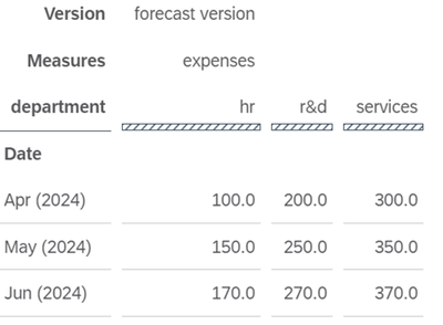
Now, let’s assume that you have created a time series forecasting model using “department” as entity dimension. A specific forecast is created for each department. When you save the forecast, values are written from April, May and June 2024, using a breakdown by department. The figure below shows the cells that are impacted when writing the forecast:
Now, the question is: how are these forecast values distributed per location?
The answer is: they are not distributed per location at all. All the values are assigned to the “Unassigned” member for the “location” dimension, as shown below:
How is that? As previously explained, the standard disaggregation behavior of the planning engine applies. Because the version was initially empty, the planning engine has no hint about how the predicted values should be spread across the different location. It falls back on the default option which is assigning the values to “Unassigned”.
This default behavior can be leveraged when you need a specific (and possibly complex) allocation logic. There are two ways to set up this allocation logic:
- Manual Approach: if you don’t need automation (typically if you need to perform the allocation only once), you can use the Distribute Value capability provided by the planning table.
- Automated Approach: if automation is required (typically if you need to perform the same allocation on a regular basis), you can create a Data Action with an allocation step describing the allocation logic you want to setup. Then you can automate the Data Action using a Multi Action. Typically, the multi actions would contain a Predictive Step to train a time series forecasting model and write the predictive forecast, followed by the Data Action for allocation.
Weighted Disaggregation
Sometimes, you don’t need complex custom allocation rules. Instead, you may want to provide disaggregation weights upfront so the planning engine can automatically disaggregate the predictive forecast. One typical use case for that, is when you want to use the weights of a comparable period to disaggregate the predictive forecast. For instance, using our expenses scenario, you may want the forecast for April-June 2024 to be allocated to the different locations using the same weights as in April-June 2023.
The disaggregation weights are provided directly as values for the forecast period in the forecast version. For instance, to force the distribution per location in April-June 2024 to be the same as in April-June 2023, you must copy the expenses values for April-June 2023 to the April-June 2024 period in your forecast version.
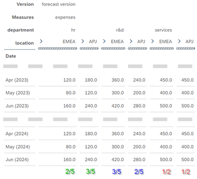
The figure below illustrates the initial state (before writing the predictive forecast) of the forecast version (the dotted lines indicate “hidden” rows so only relevant rows are visible):
We can see that April-June 2023 values have been copied to the April-June 2024 (the forecast period). Values are provided for all the “department X location” intersections so the planning engine can calculate how much of a value for a given department must go to each location. Explicitly:
- In the HR department EMEA accounts for 2/5 of the expenses, APJ accounts for the remaining 3/5.
- In the R&D department EMEA account for 3/5 of the expenses, APJ accounts for the remaining 2/5.
- In the Services department both regions account for half of the expenses.
Note that in order to keep the example simple the repartition between EMEA and APJ is constant for all the considered dates, but the repartition could as well be different depending on the date.
Now, let’s assume that you have created a time series forecasting model using “department” as entity dimension. A specific forecast is created for each department. When you save the forecast, values are written from April, May and June 2024, using a breakdown by department. The figure below shows the impacted cells:
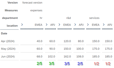
The figure below shows how the predictive forecast was automatically disaggregated per location:
We can see that the repartition of the predictive forecast per location is the same it was during the April-June 2023 period:
- In the HR department EMEA accounts for 2/5 of the expenses, APJ accounts for the remaining 3/5.
- In the R&D department EMEA account for 3/5 of the expenses, APJ accounts for the remaining 2/5.
- In the Services department both regions account for half of the expenses.
Disaggregation in Hierarchies
Disaggregation from level n to level n+1 of a hierarchy follows the rules we mentioned earlier, except when no values is available at level n+1. In such case, the value entered at level n is not allocated to the “Unassigned” value at level n+1. Instead, the level n value is spread evenly across all the level n+1 nodes (just as if the nodes in level n+1 already contained identical weights).
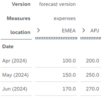
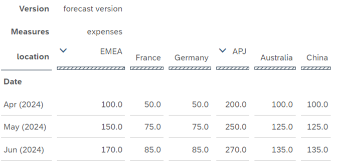
Let’s consider the “location” dimension. This dimension has a hierarchy where level 1 nodes are country groups (EMEA and APJ) and level 2 nodes are countries (France, Germany, China and Australia).
Let’s assume you want to forecast the expenses by country group (level 1).
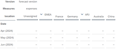
The figure below shows the initial state of the version:
The next figure shows the cells impacted when writing the predictive forecast to the forecast version:
If we expand the “location” hierarchy to show the second level, we can see that the forecast values have been disaggregated even though no disaggregation weight was initially provided:
Note again that this behavior is not specific to predictive planning: that’s just the standard disaggregation behavior of the planning engine.
Conclusion
In this blog post, you learned how to leverage the planning engine disaggregation behavior in your predictive workflows.
Do you want to learn more on Predictive Planning?
- You can also explore our learning track.
- You can also go hands-on and experience SAP Analytics Cloud by yourself.
- SAP Managed Tags:
- SAP Analytics Cloud,
- SAP Analytics Cloud for planning
You must be a registered user to add a comment. If you've already registered, sign in. Otherwise, register and sign in.
-
ABAP CDS Views - CDC (Change Data Capture)
2 -
AI
1 -
Analyze Workload Data
1 -
BTP
1 -
Business and IT Integration
2 -
Business application stu
1 -
Business Technology Platform
1 -
Business Trends
1,658 -
Business Trends
94 -
CAP
1 -
cf
1 -
Cloud Foundry
1 -
Confluent
1 -
Customer COE Basics and Fundamentals
1 -
Customer COE Latest and Greatest
3 -
Customer Data Browser app
1 -
Data Analysis Tool
1 -
data migration
1 -
data transfer
1 -
Datasphere
2 -
Event Information
1,400 -
Event Information
67 -
Expert
1 -
Expert Insights
177 -
Expert Insights
307 -
General
1 -
Google cloud
1 -
Google Next'24
1 -
GraphQL
1 -
Kafka
1 -
Life at SAP
780 -
Life at SAP
13 -
Migrate your Data App
1 -
MTA
1 -
Network Performance Analysis
1 -
NodeJS
1 -
PDF
1 -
POC
1 -
Product Updates
4,576 -
Product Updates
349 -
Replication Flow
1 -
REST API
1 -
RisewithSAP
1 -
SAP BTP
1 -
SAP BTP Cloud Foundry
1 -
SAP Cloud ALM
1 -
SAP Cloud Application Programming Model
1 -
SAP Datasphere
2 -
SAP S4HANA Cloud
1 -
SAP S4HANA Migration Cockpit
1 -
Technology Updates
6,873 -
Technology Updates
435 -
Workload Fluctuations
1
- New Machine Learning features in SAP HANA Cloud in Technology Blogs by SAP
- ML- Linear Regression definition , implementation scenarios in HANA in Technology Blogs by Members
- Forecast Local Explanation with Automated Predictive (APL) in Technology Blogs by SAP
- What’s New in SAP Analytics Cloud Release 2024.07 in Technology Blogs by SAP
- Unleashing AI and Machine Learning in Sales: Advanced Price-Volume Forecasting with SAP Analytics Cl in Technology Blogs by SAP
| User | Count |
|---|---|
| 25 | |
| 17 | |
| 11 | |
| 11 | |
| 9 | |
| 9 | |
| 9 | |
| 8 | |
| 8 | |
| 7 |

