
- SAP Community
- Products and Technology
- Technology
- Technology Blogs by SAP
- Harnessing Multi-Model Capabilities with Spotify –...
Technology Blogs by SAP
Learn how to extend and personalize SAP applications. Follow the SAP technology blog for insights into SAP BTP, ABAP, SAP Analytics Cloud, SAP HANA, and more.
Turn on suggestions
Auto-suggest helps you quickly narrow down your search results by suggesting possible matches as you type.
Showing results for
Advisor
Options
- Subscribe to RSS Feed
- Mark as New
- Mark as Read
- Bookmark
- Subscribe
- Printer Friendly Page
- Report Inappropriate Content
07-13-2023
2:50 PM
This blog is part of a series explaining the multi-model capabilities of SAP HANA Cloud /SAP Datasphere with one end-to-end scenario using Spotify data.
Here are the links for the other blogs of this series
Part 2 discussed the options of extracting, transforming, and loading JSON documents into SAP HANA Cloud and SAP Datasphere.
Now that the JSON documents are loaded and stored in SAP HANA Cloud, how about we use it for recommending the next song? In this blog, we’ll use a view created utilizing the semi structured data and use hana_ml PAL libraries to cluster the songs with similar audio features together and use it to recommend the next song.
Keep your earphones plugged as this blog will explain the following:
1. Connection to SAP HANA Cloud from Jupyter Notebook from Google Colab.
2. Exploratory Data Analysis (EDA) and data cleaning using hana_ml
3. Clustering using hana_ml
4. Song recommendation using Clustering
5. Building the Data Intelligent App
Pre-requisites:
To follow the below steps, please refer to Part 2 of the blog series to load the data from Spotify into SAP HANA Cloud and build HANA views on top of the semi structured data. Use these HANA Views as an input to the machine learning algorithm.
Dataset:
I created a view on top of all the tracks data that was ingested in Part 2.
Connection to SAP HANA Cloud from Jupyter Notebook from Google Colab:
Open the link: https://colab.research.google.com/ and create a new notebook:
You may use Jupyter Notebook from the Anaconda installed on your system.
Install the necessary libraries including hana_ml. The hana_ml package allows you to create an SAP HANA data-frame, as well as create a connection to your database instance. This package helps enable Python users to access the data-frame, build various machine learning models and run graph algorithms using the data directly from the database.
Once, the library is installed and imported in your Jupyter Notebook, you can connect to your SAP HANA Cloud system using:
Make sure the above user has access to the table/view you wish to use in your Notebook.
Create the HANA dataframe in the structure of the specified table and use .collect() to display the data in the dataframe. Please Note: there’s a difference between the HANA dataframe and Pandas dataframe
Exploratory Data Analysis:
Our data mainly consists of different audio features of songs we ingested using the Spotify APIs. Once, we have the data in the dataframe, we can explore and quantify data about music and draw valuable insights.
Let’s start by exploring our dataset using dataset_report provided by hana_ml. The DatasetReportBuilder instance can analyze the dataset and generate a report in HTML format.
Click on Sample on the left side to see a sample of the data:
To apply Machine Learnings algorithms, we need unique IDs of the songs, else, the algorithms fail to execute, to achieve that we did a drop duplicates:
After dropping the duplicates, our data is reduced from 114000 to 89741 unique records.
If we take a closer look at our data, we see that most of the features have value between 0 to 1, besides the features: tempo and loudness, so we carry out scaling features to a similar range, because normalization allows for fair comparisons between different features. It ensures that no single feature's magnitude overshadows others during analysis or modeling.
Initially, when we started this project, we did have some null values for some of the audio features. Handling null values in a Machine Learning project is an important step in the data preprocessing phase. There are various ways by which null values can be handled depending on various factors like the type of data for which we are handling null values. In our case, we handled NULL values using Imputation in which null values can be replaced with meaningful values using imputation techniques. Some common methods include replacing null values with the mean, median, mode, or a custom constant value.
After data preprocessing, let’s try to do some Exploratory Data Analysis.
To begin, let’s look at the data distribution for which we use the distribution_plot function provided by hana_ml library. It is used to visualize the distribution of a variable in a dataset. It helps in understanding the spread, shape, and characteristics of a particular feature or variable. Also, distribution_plot helps when working on feature engineering tasks, it’s crucial to understand the distribution of variables. It can help decide whether transformations like logarithmic, exponential, or power transformations are needed to normalize the data or address skewness.
We can see that the danceability, energy and valence show a normal distribution whereas acousticness, speechiness, liveness are skewed and more aligned on the lower/left side.
Next, we try to plot box plots: Box plots are used to show distributions of numeric data values, especially when you want to compare them between multiple groups. They are built to provide high-level information instantly, presenting general information about a group of data’s symmetry, skew, variance, and outliers. It is easy to see where the main bulk of the data is and make that comparison between different groups.
Both the distribution plot and box plots show that the data is skewed and there are outliers. There are various ways on how we can handle outliers like removing the data points altogether, transform the data like apply exponents or logarithmic values.
Following boxplots, we draw correlation plots, that helps to visualize the relationship or correlation between different variables in a dataset. It provides insights into how variables are related to each other correlation_plot provided by EDAVisualizer module of hana_ml.visualizers.eda or we can use the iframe generated above.
Analyzing the correlation plot, we see there’s a strong correlation between danceability and valence, which makes sense that a danceable song does make you happy!! 😊 There’s also a good correlation between energy and valence and loudness and tempo and that too aligns with our understanding: a more energetic song tends to be loud and vice-versa. Now, if we look at acousticness and energy, we see there’s negative correlation, that also makes sense, if a song has low acousticness it will consist of mostly electric sounds (think electric guitars, synthesizers, drum machines, auto-tuned vocals and so on) may have less energy.
Let’s understand the genre distribution for our dataset:
We see for our dataset, the maximum songs are in genre ‘tango’, followed by ‘study’ ,‘sleep’, ‘idm’, ‘heavy-metal’. Does that explain the distribution of acouticness?
How about drawing some correlations between audio features? Scatterplots help visualize the relationship between two variables. Scatterplots can also help reveal patterns or trends in the data. They also help identify outliers, which are data points that deviate significantly from the general pattern or trend. Please note: that scatterplot can only be drawn between two continuous variables or numerical variables.
Scatterplot between energy and loudness gives us some correlation, i.e., as loudness increases, energy increases. Pearson’s correlation plot also gave us similar idea. The plot between tempo and loudness doesn’t give us an idea that these features have some correlation. You may explore other correlation plots using the iframe created above which gives you scatter plots between all possible combinations.
The hana_ml library also provides an option to draw Word Cloud. Word clouds give visual representations of text data and the size of each word corresponds to its frequency of occurrence in the dataset. They help in understanding the most prominent or frequently occurring words in a corpus of text and provide a quick overview of the key themes. We drew Word Cloud for the genres and track names from our dataset.
Song Recommendation:
The idea was not to build a recommendation system to compete or draw a parallel with all the recommendation systems that exist, but to show the capabilities of SAP HANA Cloud multi-modeling features.
To build the recommendation system, the idea is to cluster the songs together using the clustering algorithms provides by hana_ml on the data stored in SAP HANA Cloud. There are a variety of clustering algorithms provided by hana_ml and the documentation for the same can be found here.
Before, writing and executing the code for the Machine Learning algorithm, activate the SQL trace in SAP HANA Cloud, which will be needed later for building the SAP Intelligent Data application.
Let’s follow the below steps to build the data intelligent apps, the first part is to build the song recommendation.
Building Data Intelligent Application
Intelligent Data apps help embed data science and machine learning to enhance business processes, converge multiple data types in a unified database. The very foundation of building Intelligent Data Application is the Out of the box Machine Learning with SAP HANA Cloud.
Looking at the approach of building the Intelligent Data Application, we need to follow the below steps:
Before, we delve any deeper to the algorithms and machine learning implementation, let’s understand SAP’s machine learning offering. SAP HANA offers SAP PAL (Predictive Analytics Library) which is a component of the SAP HANA platform that provides a set of advanced predictive and machine learning algorithms. It offers a wide range of algorithms for various analytical use cases, including regression, classification, clustering, time series analysis, and more. Its basic benefit is it’s integration with SAP HANA and In-Database processing since these algorithms are executed directly on SAP HANA, without having to move the data around. You can use PAL procedures through the Python and R machine learning clients for SAP HANA. For our project, we chose to use PAL procedures through Python.
For song recommendation system, we are using KMeans clustering algorithm. It aims to partition a dataset into K distinct clusters based on the similarity of data points. The K-means algorithm aims to minimize the within-cluster sum of squared distances, which means that data points within the same cluster are alike each other compared to data points in different clusters. The choice of K, the number of clusters, is an important parameter that needs to be determined beforehand. For our project, we iterated from 4 clusters to 7 clusters and found 5 to work the best.
To begin with the ML algorithm, we split the dataset into test and train:
Created an instance of KMeans using:
Next, we must use t-SNE (t-Distributed Stochastic Neighbor Embedding) technique, which is a dimensionality reduction technique used for visualizing high-dimensional data in a lower-dimensional space. It is particularly effective in visualizing complex, nonlinear patterns in the data. The main idea behind t-SNE is to map each data point from its high-dimensional space to a low-dimensional space (usually 2D or 3D). While preserving the pairwise similarities between the points as much as possible. It achieves this by modeling the similarity between data points in the high-dimensional space and the low-dimensional space using a probabilistic approach. In the context of Spotify audio features, the term "dimension" typically refers to the number of numerical features or attributes associated with each audio track.
The above process is a time taking process and depends on the number of iterations. The number of iterations in t-SNE (t-Distributed Stochastic Neighbor Embedding) algorithm can impact the quality of the embedding and the computational time required. The optimal number of iterations depends on the dataset, its complexity, and the desired level of accuracy.
Once, the algorithm execution completes, we receive the output in two dimensions as follows which is perfect for us to plot in 2D space:
Using the library plotly express, we plotted the clusters in 2D space as follows:
We see that our songs are clustered into five clusters. If you hover on the points, you’d the genre and the track name as well.
To begin with understanding how we built a recommendation system, let’s understand a little about recommendations. Recommendations refer to the process of suggesting items or content to users based on their preferences, historical behavior, or similarity to other users. The goal of recommendations is to provide personalized and relevant suggestions to enhance user experiences, facilitate discovery, and increase engagement. Recommendations can be personalized, collaborative (based on similar users), content-based (based on item attributes)
Based on the analysis and visualizations, it’s clear that songs with similar audio features tend to have data points that are located close to each other. This observation makes perfect sense. We have used this same idea to build a recommendation system using SAP HANA Cloud by taking the data points of the songs a user has listened to and recommending songs corresponding to nearby data points the information for which we get from the songs clustered together. Cluster the songs together, and when a user requests recommendations, identify the cluster(s) that the song belongs with and retrieve songs closest to the song that user requested based on the distance and recommend those songs to the user.
Testing the recommendations:
We have already completed the Build part where we used KMeans machine learning algorithm and based on that model, we build a method which helps recommend songs based on the distance closest the song chosen all using hana_ml and data also stored on HANA.
Now, let’s Generate the design-time artifacts for machine learning scenario with the help of hana_ml library. To achieve that, we use the hana_ml.artifacts.generators.hana module in hana_ml. This module handles generation of all HANA design-time artifacts based on the provided base and consumption layer elements. These artifacts can be incorporated into development projects in SAP Web IDE for SAP HANA or SAP Business Application Studio and be deployed via HANA Deployment Infrastructure (HDI) into a SAP HANA Cloud system. The HANAGeneratorForCAP automatically generates the procedures, grants, CAP cds entities with corresponding signatures. This eases the job of a developer having to manually create these artifacts from scratch to embed intelligence in the apps.
Expanding the folder, we see we have .hdbgrants file generated which would contain the grants for the object owner user of the HDI container, the .hdbsynonym would contain the synonyms for all the objects which are outside the container, for example: _SYS_AFL schema. There are two procedures which are created which call the _SYS_AFL.PALKMEANS algorithm/procedure. The base procedure calls the algorithm and cons is for the end consumption used for calling the training and the inference in the target system. This generation was possible when the SQL trace is enabled on the SAP HANA Cloud instance which we had enabled initially.
Now that the artifacts are generated, we need to Develop a full stack application using Business Application Studio. Before we start the development, we need to create a user and assign the following privileges. This user acts as the technical user for the user-provided-service. The user can either be created using the command below or using the SAP HANA Cloud Cockpit":
Create a user:
--create user
CREATE USER PAL_ACCESS PASSWORD <> NO FORCE_FIRST_PASSWORD CHANGE;
--create roles
CREATE ROLE "data::external_access_g";
CREATE ROLE "data::external_access";
--assign roles to the newly created user, additionally assign the ROLE ADMIN SYSTEM privilege.
GRANT "data::external_access_g", "data::external_access" TO PAL_ACCESS WITH ADMIN OPTION;
GRANT ROLE ADMIN TO PAL_ACCESS.
-- assign AFL roles with GRANT option to the newly created user.
GRANT AFL__SYS_AFL_AFLPAL_EXECUTE_WITH_GRANT_OPTION, AFL__SYS_AFL_AFLPAL_EXECUTE_WITH_GRANT_OPTION to "data::external_access_g";
GRANT AFL__SYS_AFL_AFLPAL_EXECUTE, AFL__SYS_AFL_AFLPAL_EXECUTE_WITH_GRANT_OPTION to "data::external_access";
Use the same user and create the user-provided service. This user-provided service provides the necessary authorization to the runtime HDI user to run machine learning models which are a part of _SYS_AFL schema in HANA.
Create the user-provided-service:
Go to the space where your SAP HANA Cloud application will be created and in instances Create -> User-Provided Service Instance.
Provide the syntax as follows:
Create CAP application:
There are multiple steps involved in building the CAP application:
Dev Space: Create a new Full Stack Cloud Application Dev Space in Business Application Studio or use the one you may already have.
Create a new application from Template and enter the details and click Finish:
New application is created in your Business Application Studio:
Upload the generated files to respective folders as below:
Open the terminal and do a cds build. This generates the artifacts specified in the ‘hana-ml-cds-hana-ml-base-pal-kmeans.cds’ and generates the views and tables specified in the .cds file.
Deploy the generated artifacts:
Bind the user-provided-service by adding it in the mta.yaml as follows:
Click on Bind:
Change the user-provided service in .hdbgrants as follows:
Bind the HDI container:
As you may have seen, the .hdbsynonym file is automatically generated for you which contains the synonym for the _SYS_AFL, a schema that provides us with the PAL algorithms. Since, our algorithm also makes use of other tables/views stored in SAP HANA Cloud which are not a part of this container, we need to create a synonym for the same. Build all the other artifacts including the procedures, grants and synonym files.
The generated HDI artifacts are now successfully built in the container. To make the consumption of the recommendation method easier, we created a wrapper procedure around the *cons* procedure which we’ll use as a function in our OData service. To achieve this, we created two more artifacts: another entity in the hana-ml-cds-hana-ml-base-pal-kmeans.cds file and a recommendnextsong.hdbprocedure as follows:
We have now completed our HANA development, let’s start with the development of the app. For the app, the Catalog service: hana-ml-cat-service.cds is already generated for us by the HANAGeneratorForCAP module, where we added two entries as below and to handle this we now need to build the hana-ml-cat-service.js. Make sure, the handler has the same name as the catalog service file.
If you wish to have a Fiori preview, then add the following code to the project’s package.json file as follows:
Test/Consume the application created:
All our artifacts are built and successfully deployed, next step is to test the application and consume it. We could deploy the full stack application to BTP and consume it from the BTP portal or we could do a quick test within the BAS with the following steps:
Open the link that’s prompted and we can either open the OData service or the Fiori preview:
Click on $metadata and test it with an ID:
https://<yourappsurl>/catalog/recommendnextsong(ID='6vCzWS8xkRbilNXuwvuQ7O')
We can see our recommendations!! 😊
We can choose to save our model in SAP HANA Cloud for referring it to it later:
We can also choose to store the results of recommendations in our SAP Datasphere instance:
Go to your SAP Datasphere instance, open Space Management and create a new user. Get the details of your instance like host, user and password.
In your Jupyter Notebook, create a connection to your SAP Datasphere instance and create the dataframe using HANA_ML library.
You can now create a view on top of the table in your SAP Datasphere:
With that, I finish this blog, let me know your thoughts!
Here are the links for the other blogs of this series
- Part 1 – Architecture
- Part 2 – Processing Semi-Structured data in SAP HANA Cloud
- Part 3 – Processing Semi-structured data in SAP Datasphere
- Part 4 – Processing Semi-structured data for SAP HANA Graph
Part 2 discussed the options of extracting, transforming, and loading JSON documents into SAP HANA Cloud and SAP Datasphere.
Now that the JSON documents are loaded and stored in SAP HANA Cloud, how about we use it for recommending the next song? In this blog, we’ll use a view created utilizing the semi structured data and use hana_ml PAL libraries to cluster the songs with similar audio features together and use it to recommend the next song.
Keep your earphones plugged as this blog will explain the following:
1. Connection to SAP HANA Cloud from Jupyter Notebook from Google Colab.
2. Exploratory Data Analysis (EDA) and data cleaning using hana_ml
3. Clustering using hana_ml
4. Song recommendation using Clustering
5. Building the Data Intelligent App
Pre-requisites:
To follow the below steps, please refer to Part 2 of the blog series to load the data from Spotify into SAP HANA Cloud and build HANA views on top of the semi structured data. Use these HANA Views as an input to the machine learning algorithm.
Dataset:
I created a view on top of all the tracks data that was ingested in Part 2.
Connection to SAP HANA Cloud from Jupyter Notebook from Google Colab:
Open the link: https://colab.research.google.com/ and create a new notebook:

Open Jupyter Notebook from Google Colab
You may use Jupyter Notebook from the Anaconda installed on your system.
Install the necessary libraries including hana_ml. The hana_ml package allows you to create an SAP HANA data-frame, as well as create a connection to your database instance. This package helps enable Python users to access the data-frame, build various machine learning models and run graph algorithms using the data directly from the database.
Once, the library is installed and imported in your Jupyter Notebook, you can connect to your SAP HANA Cloud system using:

Connect your SAP HANA Cloud instance
Make sure the above user has access to the table/view you wish to use in your Notebook.
Create the HANA dataframe in the structure of the specified table and use .collect() to display the data in the dataframe. Please Note: there’s a difference between the HANA dataframe and Pandas dataframe

Exploratory Data Analysis:
Our data mainly consists of different audio features of songs we ingested using the Spotify APIs. Once, we have the data in the dataframe, we can explore and quantify data about music and draw valuable insights.
Let’s start by exploring our dataset using dataset_report provided by hana_ml. The DatasetReportBuilder instance can analyze the dataset and generate a report in HTML format.

Create your EDA in HTML report format

Dataset Report generated on the dataset used
Click on Sample on the left side to see a sample of the data:

Sample of the dataset used
To apply Machine Learnings algorithms, we need unique IDs of the songs, else, the algorithms fail to execute, to achieve that we did a drop duplicates:
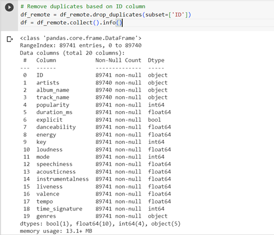
Duplicated dropped from dataset
After dropping the duplicates, our data is reduced from 114000 to 89741 unique records.
If we take a closer look at our data, we see that most of the features have value between 0 to 1, besides the features: tempo and loudness, so we carry out scaling features to a similar range, because normalization allows for fair comparisons between different features. It ensures that no single feature's magnitude overshadows others during analysis or modeling.

Normalization of dataset columns
Initially, when we started this project, we did have some null values for some of the audio features. Handling null values in a Machine Learning project is an important step in the data preprocessing phase. There are various ways by which null values can be handled depending on various factors like the type of data for which we are handling null values. In our case, we handled NULL values using Imputation in which null values can be replaced with meaningful values using imputation techniques. Some common methods include replacing null values with the mean, median, mode, or a custom constant value.
Imputation helps to maintain the overall structure of the dataset by filling in missing values. The reason we chose Imputation is because we wanted to handle the null audio features which were numerical in nature.
Imputation of dataset columns
After data preprocessing, let’s try to do some Exploratory Data Analysis.
To begin, let’s look at the data distribution for which we use the distribution_plot function provided by hana_ml library. It is used to visualize the distribution of a variable in a dataset. It helps in understanding the spread, shape, and characteristics of a particular feature or variable. Also, distribution_plot helps when working on feature engineering tasks, it’s crucial to understand the distribution of variables. It can help decide whether transformations like logarithmic, exponential, or power transformations are needed to normalize the data or address skewness.
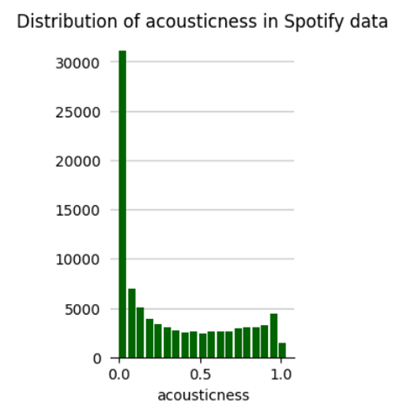


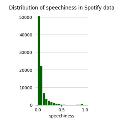


We can see that the danceability, energy and valence show a normal distribution whereas acousticness, speechiness, liveness are skewed and more aligned on the lower/left side.
Next, we try to plot box plots: Box plots are used to show distributions of numeric data values, especially when you want to compare them between multiple groups. They are built to provide high-level information instantly, presenting general information about a group of data’s symmetry, skew, variance, and outliers. It is easy to see where the main bulk of the data is and make that comparison between different groups.
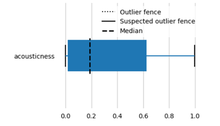


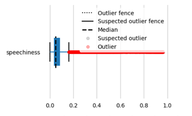


Both the distribution plot and box plots show that the data is skewed and there are outliers. There are various ways on how we can handle outliers like removing the data points altogether, transform the data like apply exponents or logarithmic values.
Following boxplots, we draw correlation plots, that helps to visualize the relationship or correlation between different variables in a dataset. It provides insights into how variables are related to each other correlation_plot provided by EDAVisualizer module of hana_ml.visualizers.eda or we can use the iframe generated above.

Pearsons correlation plot
Analyzing the correlation plot, we see there’s a strong correlation between danceability and valence, which makes sense that a danceable song does make you happy!! 😊 There’s also a good correlation between energy and valence and loudness and tempo and that too aligns with our understanding: a more energetic song tends to be loud and vice-versa. Now, if we look at acousticness and energy, we see there’s negative correlation, that also makes sense, if a song has low acousticness it will consist of mostly electric sounds (think electric guitars, synthesizers, drum machines, auto-tuned vocals and so on) may have less energy.
Let’s understand the genre distribution for our dataset:

Genre Distribution
We see for our dataset, the maximum songs are in genre ‘tango’, followed by ‘study’ ,‘sleep’, ‘idm’, ‘heavy-metal’. Does that explain the distribution of acouticness?
How about drawing some correlations between audio features? Scatterplots help visualize the relationship between two variables. Scatterplots can also help reveal patterns or trends in the data. They also help identify outliers, which are data points that deviate significantly from the general pattern or trend. Please note: that scatterplot can only be drawn between two continuous variables or numerical variables.
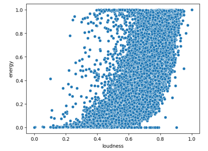
Scatterplot for energy and loudness
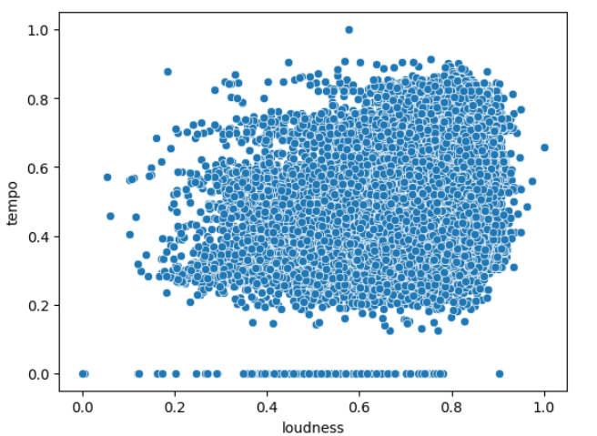
Scatterplot for tempo and loudness
Scatterplot between energy and loudness gives us some correlation, i.e., as loudness increases, energy increases. Pearson’s correlation plot also gave us similar idea. The plot between tempo and loudness doesn’t give us an idea that these features have some correlation. You may explore other correlation plots using the iframe created above which gives you scatter plots between all possible combinations.
The hana_ml library also provides an option to draw Word Cloud. Word clouds give visual representations of text data and the size of each word corresponds to its frequency of occurrence in the dataset. They help in understanding the most prominent or frequently occurring words in a corpus of text and provide a quick overview of the key themes. We drew Word Cloud for the genres and track names from our dataset.


Word Cloud for genres and track names
Song Recommendation:
The idea was not to build a recommendation system to compete or draw a parallel with all the recommendation systems that exist, but to show the capabilities of SAP HANA Cloud multi-modeling features.
To build the recommendation system, the idea is to cluster the songs together using the clustering algorithms provides by hana_ml on the data stored in SAP HANA Cloud. There are a variety of clustering algorithms provided by hana_ml and the documentation for the same can be found here.
Before, writing and executing the code for the Machine Learning algorithm, activate the SQL trace in SAP HANA Cloud, which will be needed later for building the SAP Intelligent Data application.
Let’s follow the below steps to build the data intelligent apps, the first part is to build the song recommendation.
Building Data Intelligent Application
Intelligent Data apps help embed data science and machine learning to enhance business processes, converge multiple data types in a unified database. The very foundation of building Intelligent Data Application is the Out of the box Machine Learning with SAP HANA Cloud.
Looking at the approach of building the Intelligent Data Application, we need to follow the below steps:

Steps to build Intelligent Data Application
- Build
Before, we delve any deeper to the algorithms and machine learning implementation, let’s understand SAP’s machine learning offering. SAP HANA offers SAP PAL (Predictive Analytics Library) which is a component of the SAP HANA platform that provides a set of advanced predictive and machine learning algorithms. It offers a wide range of algorithms for various analytical use cases, including regression, classification, clustering, time series analysis, and more. Its basic benefit is it’s integration with SAP HANA and In-Database processing since these algorithms are executed directly on SAP HANA, without having to move the data around. You can use PAL procedures through the Python and R machine learning clients for SAP HANA. For our project, we chose to use PAL procedures through Python.
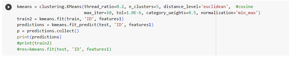
For song recommendation system, we are using KMeans clustering algorithm. It aims to partition a dataset into K distinct clusters based on the similarity of data points. The K-means algorithm aims to minimize the within-cluster sum of squared distances, which means that data points within the same cluster are alike each other compared to data points in different clusters. The choice of K, the number of clusters, is an important parameter that needs to be determined beforehand. For our project, we iterated from 4 clusters to 7 clusters and found 5 to work the best.
To begin with the ML algorithm, we split the dataset into test and train:
![]()
Created an instance of KMeans using:
Next, we must use t-SNE (t-Distributed Stochastic Neighbor Embedding) technique, which is a dimensionality reduction technique used for visualizing high-dimensional data in a lower-dimensional space. It is particularly effective in visualizing complex, nonlinear patterns in the data. The main idea behind t-SNE is to map each data point from its high-dimensional space to a low-dimensional space (usually 2D or 3D). While preserving the pairwise similarities between the points as much as possible. It achieves this by modeling the similarity between data points in the high-dimensional space and the low-dimensional space using a probabilistic approach. In the context of Spotify audio features, the term "dimension" typically refers to the number of numerical features or attributes associated with each audio track.

The above process is a time taking process and depends on the number of iterations. The number of iterations in t-SNE (t-Distributed Stochastic Neighbor Embedding) algorithm can impact the quality of the embedding and the computational time required. The optimal number of iterations depends on the dataset, its complexity, and the desired level of accuracy.
Once, the algorithm execution completes, we receive the output in two dimensions as follows which is perfect for us to plot in 2D space:

Using the library plotly express, we plotted the clusters in 2D space as follows:

Obtained five clusters as a result of KMeans machine learning algorithm
We see that our songs are clustered into five clusters. If you hover on the points, you’d the genre and the track name as well.
To begin with understanding how we built a recommendation system, let’s understand a little about recommendations. Recommendations refer to the process of suggesting items or content to users based on their preferences, historical behavior, or similarity to other users. The goal of recommendations is to provide personalized and relevant suggestions to enhance user experiences, facilitate discovery, and increase engagement. Recommendations can be personalized, collaborative (based on similar users), content-based (based on item attributes)

Types of recommendation systems: source: KNuggets
Based on the analysis and visualizations, it’s clear that songs with similar audio features tend to have data points that are located close to each other. This observation makes perfect sense. We have used this same idea to build a recommendation system using SAP HANA Cloud by taking the data points of the songs a user has listened to and recommending songs corresponding to nearby data points the information for which we get from the songs clustered together. Cluster the songs together, and when a user requests recommendations, identify the cluster(s) that the song belongs with and retrieve songs closest to the song that user requested based on the distance and recommend those songs to the user.

Recommend songs
Testing the recommendations:

- Generate the design time artifacts:
We have already completed the Build part where we used KMeans machine learning algorithm and based on that model, we build a method which helps recommend songs based on the distance closest the song chosen all using hana_ml and data also stored on HANA.
Now, let’s Generate the design-time artifacts for machine learning scenario with the help of hana_ml library. To achieve that, we use the hana_ml.artifacts.generators.hana module in hana_ml. This module handles generation of all HANA design-time artifacts based on the provided base and consumption layer elements. These artifacts can be incorporated into development projects in SAP Web IDE for SAP HANA or SAP Business Application Studio and be deployed via HANA Deployment Infrastructure (HDI) into a SAP HANA Cloud system. The HANAGeneratorForCAP automatically generates the procedures, grants, CAP cds entities with corresponding signatures. This eases the job of a developer having to manually create these artifacts from scratch to embed intelligence in the apps.
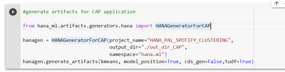
Generate artifacts for CAP application

Generated artifacts
Expanding the folder, we see we have .hdbgrants file generated which would contain the grants for the object owner user of the HDI container, the .hdbsynonym would contain the synonyms for all the objects which are outside the container, for example: _SYS_AFL schema. There are two procedures which are created which call the _SYS_AFL.PALKMEANS algorithm/procedure. The base procedure calls the algorithm and cons is for the end consumption used for calling the training and the inference in the target system. This generation was possible when the SQL trace is enabled on the SAP HANA Cloud instance which we had enabled initially.
- Develop
Now that the artifacts are generated, we need to Develop a full stack application using Business Application Studio. Before we start the development, we need to create a user and assign the following privileges. This user acts as the technical user for the user-provided-service. The user can either be created using the command below or using the SAP HANA Cloud Cockpit":
Create a user:
--create user
CREATE USER PAL_ACCESS PASSWORD <> NO FORCE_FIRST_PASSWORD CHANGE;
--create roles
CREATE ROLE "data::external_access_g";
CREATE ROLE "data::external_access";
--assign roles to the newly created user, additionally assign the ROLE ADMIN SYSTEM privilege.
GRANT "data::external_access_g", "data::external_access" TO PAL_ACCESS WITH ADMIN OPTION;
GRANT ROLE ADMIN TO PAL_ACCESS.
-- assign AFL roles with GRANT option to the newly created user.
GRANT AFL__SYS_AFL_AFLPAL_EXECUTE_WITH_GRANT_OPTION, AFL__SYS_AFL_AFLPAL_EXECUTE_WITH_GRANT_OPTION to "data::external_access_g";
GRANT AFL__SYS_AFL_AFLPAL_EXECUTE, AFL__SYS_AFL_AFLPAL_EXECUTE_WITH_GRANT_OPTION to "data::external_access";
Use the same user and create the user-provided service. This user-provided service provides the necessary authorization to the runtime HDI user to run machine learning models which are a part of _SYS_AFL schema in HANA.
Create the user-provided-service:
Go to the space where your SAP HANA Cloud application will be created and in instances Create -> User-Provided Service Instance.
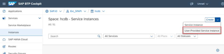
BTP Cockpit services
Provide the syntax as follows:

user-provided service in BTP
Create CAP application:
There are multiple steps involved in building the CAP application:
Dev Space: Create a new Full Stack Cloud Application Dev Space in Business Application Studio or use the one you may already have.
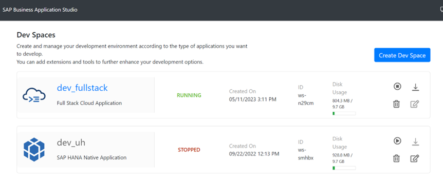
BAS Dev spaces
Create a new application from Template and enter the details and click Finish:
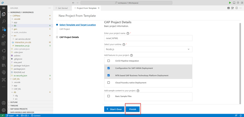
Create Full Stack application from template
New application is created in your Business Application Studio:
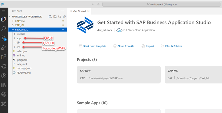
Newly created project in BAS workspace
Upload the generated files to respective folders as below:

Uploaded generated files to the project
Open the terminal and do a cds build. This generates the artifacts specified in the ‘hana-ml-cds-hana-ml-base-pal-kmeans.cds’ and generates the views and tables specified in the .cds file.

cds build for generated artifacts

Log of cds build
Deploy the generated artifacts:

Deploy the generated artifacts

deployed artifacts
Bind the user-provided-service by adding it in the mta.yaml as follows:

Add ups to mta.yaml

user provided service is now a part of the project
Click on Bind:

bind the ups
Change the user-provided service in .hdbgrants as follows:

adjust the .hdbgrants with the correct ups name
Bind the HDI container:


As you may have seen, the .hdbsynonym file is automatically generated for you which contains the synonym for the _SYS_AFL, a schema that provides us with the PAL algorithms. Since, our algorithm also makes use of other tables/views stored in SAP HANA Cloud which are not a part of this container, we need to create a synonym for the same. Build all the other artifacts including the procedures, grants and synonym files.

.hdbsynonym for the HDI module
The generated HDI artifacts are now successfully built in the container. To make the consumption of the recommendation method easier, we created a wrapper procedure around the *cons* procedure which we’ll use as a function in our OData service. To achieve this, we created two more artifacts: another entity in the hana-ml-cds-hana-ml-base-pal-kmeans.cds file and a recommendnextsong.hdbprocedure as follows:


Wrapper .hdbprocedure
We have now completed our HANA development, let’s start with the development of the app. For the app, the Catalog service: hana-ml-cat-service.cds is already generated for us by the HANAGeneratorForCAP module, where we added two entries as below and to handle this we now need to build the hana-ml-cat-service.js. Make sure, the handler has the same name as the catalog service file.

Service Catalog
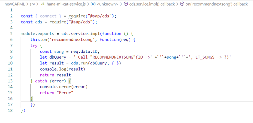
Handler of service catalog
If you wish to have a Fiori preview, then add the following code to the project’s package.json file as follows:

Test/Consume the application created:
All our artifacts are built and successfully deployed, next step is to test the application and consume it. We could deploy the full stack application to BTP and consume it from the BTP portal or we could do a quick test within the BAS with the following steps:


run the application from BAS terminal
Open the link that’s prompted and we can either open the OData service or the Fiori preview:
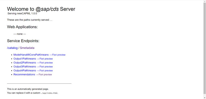
Click on $metadata and test it with an ID:
https://<yourappsurl>/catalog/recommendnextsong(ID='6vCzWS8xkRbilNXuwvuQ7O')

Results of recommendations
We can see our recommendations!! 😊
We can choose to save our model in SAP HANA Cloud for referring it to it later:
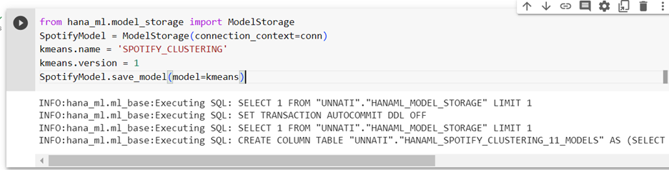
Model storage
We can also choose to store the results of recommendations in our SAP Datasphere instance:
Go to your SAP Datasphere instance, open Space Management and create a new user. Get the details of your instance like host, user and password.

SAP Datasphere creation of user
In your Jupyter Notebook, create a connection to your SAP Datasphere instance and create the dataframe using HANA_ML library.

Store inference results in SAP Datasphere
You can now create a view on top of the table in your SAP Datasphere:
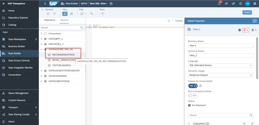
Use the inference results in SAP Datasphere
With that, I finish this blog, let me know your thoughts!
- SAP Managed Tags:
- Machine Learning,
- SAP Datasphere,
- SAP HANA Cloud,
- SAP HANA multi-model processing
Labels:
2 Comments
You must be a registered user to add a comment. If you've already registered, sign in. Otherwise, register and sign in.
Labels in this area
-
ABAP CDS Views - CDC (Change Data Capture)
2 -
AI
1 -
Analyze Workload Data
1 -
BTP
1 -
Business and IT Integration
2 -
Business application stu
1 -
Business Technology Platform
1 -
Business Trends
1,658 -
Business Trends
93 -
CAP
1 -
cf
1 -
Cloud Foundry
1 -
Confluent
1 -
Customer COE Basics and Fundamentals
1 -
Customer COE Latest and Greatest
3 -
Customer Data Browser app
1 -
Data Analysis Tool
1 -
data migration
1 -
data transfer
1 -
Datasphere
2 -
Event Information
1,400 -
Event Information
67 -
Expert
1 -
Expert Insights
177 -
Expert Insights
301 -
General
1 -
Google cloud
1 -
Google Next'24
1 -
GraphQL
1 -
Kafka
1 -
Life at SAP
780 -
Life at SAP
13 -
Migrate your Data App
1 -
MTA
1 -
Network Performance Analysis
1 -
NodeJS
1 -
PDF
1 -
POC
1 -
Product Updates
4,577 -
Product Updates
346 -
Replication Flow
1 -
REST API
1 -
RisewithSAP
1 -
SAP BTP
1 -
SAP BTP Cloud Foundry
1 -
SAP Cloud ALM
1 -
SAP Cloud Application Programming Model
1 -
SAP Datasphere
2 -
SAP S4HANA Cloud
1 -
SAP S4HANA Migration Cockpit
1 -
Technology Updates
6,873 -
Technology Updates
429 -
Workload Fluctuations
1
Related Content
- Quick & Easy Datasphere - When to use Data Flow, Transformation Flow, SQL View? in Technology Blogs by Members
- Exploring Integration Options in SAP Datasphere with the focus on using SAP extractors - Part II in Technology Blogs by SAP
- New Machine Learning features in SAP HANA Cloud in Technology Blogs by SAP
- 10+ ways to reshape your SAP landscape with SAP Business Technology Platform – Blog 4 in Technology Blogs by SAP
- Top Picks: Innovations Highlights from SAP Business Technology Platform (Q1/2024) in Technology Blogs by SAP
Top kudoed authors
| User | Count |
|---|---|
| 34 | |
| 17 | |
| 15 | |
| 14 | |
| 11 | |
| 9 | |
| 8 | |
| 8 | |
| 8 | |
| 7 |