
- SAP Community
- Products and Technology
- Financial Management
- Financial Management Blogs by SAP
- How to transform your SAP S/4HANA system in a mach...
Financial Management Blogs by SAP
Get financial management insights from blog posts by SAP experts. Find and share tips on how to increase efficiency, reduce risk, and optimize working capital.
Turn on suggestions
Auto-suggest helps you quickly narrow down your search results by suggesting possible matches as you type.
Showing results for
Employee
Options
- Subscribe to RSS Feed
- Mark as New
- Mark as Read
- Bookmark
- Subscribe
- Printer Friendly Page
- Report Inappropriate Content
06-10-2018
8:05 AM
In this blog, explain how you can use your SAP S/4HANA system to execute machine learning tasks. We sketch a step-by-step guide on how to process the data, execute the relevant database procedure and discuss potential ways to expose the results. The advantages of this approach are that no data replication is needed and the use of database procedures offer great performance. Note that this approach requires custom development on the S/4HANA system.
You may wonder why you want to do machine learning on an S/4HANA System? If you search the internet, you realize that Python based libraries like scikit-learn, pandas etc. and frameworks as Jupyter have become the standard in the ML community. They are easy to use and offer a low entry barrier, a comfortable learning curve and a big community.However, in some cases you cannot use this kind of tooling.
We wanted to include an anomaly detection for suspicious expenses in our finance application, SAP RealSpend [1], that visualizes lots of expense data. Scanning the thousands of entries by hand is very cumbersome and error prone. An automatic detection of suspicious entries would be of great value for the user. The application is extension to S/4HANA and runs on the SAP Cloud Platform (SCP). Users subscribe to the application and pay on a per-user, per-month basis.
With this scenario in mind, some architectural choices are unavoidable. The replication of sensitive financial data to the SCP is critical, because we guarantee our customers, that no data is leaving their ERP and the SCP works like a proxy
SAP offers dedicated data platforms, which offer data replication and ML in a secure way [2]. As we want to keep the entrance conditions to use SAP RealSpend as a subscription based and easy to install extension as low as possible, requiring the customer to have a datahub in place is not an option at the moment.
Keeping these boundary conditions in mind, we realized that we should bring the algorithm to the data. Luckily the S/4HANA system offers the predictive analytic library [3], that provides a large set of fast database (DB) procedures to perform standard ML tasks like clustering, interpolation and model training. The DB procedures are called via SQLScript, but no worries, there is no need to create large scripts: The ABAP stack provides so called ABAP managed database procedures (AMDP). These objects work as an intersection between the ABAP and SQLScript stack. In our implementation, we did as much as possible in the strongly typed ABAP and only very little in SQLScript. We will come to the implementation details later.
For the exposure of the functionality we created an OData service. This service provides endpoints to train and then make predictions for trained models.
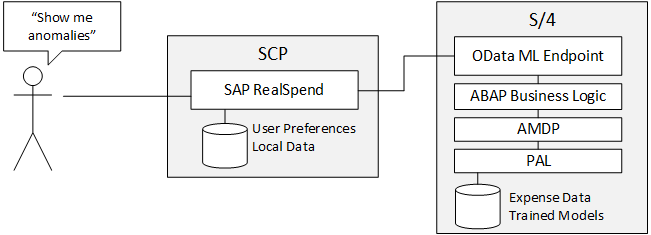
Figure 1: High level architecture of the ML feature in RealSpend.
The problem we wanted to solve is very easy to define: “Show me suspicious entries in the ACDOCA table of the S/4HANA system”. As often in life, simple questions are not easy to answer. There are whole books on anomaly detection [4] and we started to look for an “out of the box” solution for the problem. The problem with expense anomalies is, that you need some domain knowledge to find anomalies. The problem is as universal as for example pattern recognition. The question was how to proceed from here? In our case we find the following approach fruitful:
The speed for iterations is much faster in Python. Hence, we really recommend trying things in Python first and after you verified it is working implement it in ABAP. There is a Florian [5] which covers the problem of finding anomalies. Here we will briefly present one simple approach we found and then implemented in the S/4HANA system.
Since we did not have a big set of already classified data supervised learning was not an option. As a first step we needed to find a simple approach to automatically classify the expenses as “anomaly” and “no anomaly”.
The idea is to use clustering of expenses to find entries which are isolated. Clustering all expenses together was not leading good results, salaries. Hence, we used the account (RAACT on ACDOCA) to naturally group expenses and did the clustering by account. Additionally, we realized that the amounts depended on the person (PERNR on ACDOCA). A high-level manager has a higher spending level for travel then an associate developer. To summarize, we did the clustering in the following way:

Figure 2: Result of the clustering. Anomalies are colored orange. The density of all expense entries (right) does not show solitary entries. The second feature PerNr makes them visible.
We used DBSCAN for clustering for multiple reasons:
Having this algorithm in place the initial labeling of the data is done. Up to know nothing fancy has happened. You could call this machine learning, we’d rather call it statistics.
The magic happens in the next step. The labeled data is used to train a classification model like a random decision tree. Having a trained model has multiple advantages:
Over time the prediction quality of the model will decrease, because more and more entries enter the system, which have not been considered in the initial labeling. Hence it is important to implement a retrain condition which triggers a retraining after a certain amount of time.
After discussing all the theory, we now want to share some implementation details, which will help you to realize your ML use case. The first part was the exposure of the functionality via a custom OData service. First you build the data model in the SEGW. We used a model entity to manage the different model related actions. Note that the model entity has the following properties:

Figure 3: Entity builder for our ML case.
The calculation entity takes a model as an input and provides the prediction. Currently this functionality is disabled, because we are waiting for the general model managing package SHEMI is available on S/4HANA. However, the initial labeling from the model endpoint is fast enough to be called without storing the model. You implement the data provider and model provider class as usual to handle your request.
As discussed, the selected data must be processed: group by accounts, remove groups with too small size, calculate the median per person. We will not discuss the implementation details in this blog. The general idea was to implement as much as possible in ABAP. For example, the calculation of the median can be done very efficiently using the GROUP BY keyword:

Figure 4: Example for the data processing.
It is a good idea to write tests while developing or even start with the tests. To make the code independent from the underlying system, the necessary test data with our development. In this context test data containers (TDC) are a useful feature.

Figure 5: Test data container containing the test data.
The TDCs are development objects and are part of the standard ABAP transport system. In our tests we read the test container data using the test data container API. You can have a look at the class cl_apl_ecatt_tdc_api, which provides the necessary methods. In the example above, you see an entry in line 8 which has an amount of 10. This is significantly bigger than the other values for this person with PERNR Per1. So, the clustering should return this value as a single separate cluster.
Congratulations, you have arrived at the machine learning part. Up to now we have talked about how we exposed the service and how to process and prepare the data for the clustering. Now it is time to do the clustering. From our tests in the Python framework we found that DBSCAN works nicely and estimated the parameters for this clustering.
For DBSCAN there is already a predefined DB procedure SYSAFL.paldbscan we used for this task. The procedure is called via ABAP managed database procedures (AMDP) which is a wrapper for SQLScript:
As discussed in the previous section we do all the data preparation in ABAP. In the it_pal_control table the parameters cluster size & bandwidth are given and it_data contains the data for the clustering in the form:
We choose the data types of the data structure in accordance to the mapping of ABAP and SQLScript types [6]. Doing so, it is guaranteed that the values are properly casted when they are passed from the ABAP to the SQLScript layer.
Note that AMDP procedures only support call by value and a local database table is created on the fly while calling the AMDP. If you want to avoid this overhead you could only pass the selection criteria in your AMDP method and do the data collection and processing within SQLScript. This would reduce the amount of memory consumption and memory allocation but force you to implement logic in an untyped language. Since we never faced performance issues in our tests we did not pursue this optimization.
Once you have the initial labeling of the expense via the DBSCAN we train our model. We found that a random decision tree works well:
The input is self-explaining. It is important that you pass at least all features used for the initial labeling process to get meaningful results. In our case the amount, person number and account. At this point it would be easy to include some user feedback and labeling related to other automatic classification approaches. The final model contains then typical decision tree conditions:

Figure 6: Part of a decision tree.
You can persist the content of et_model for later usage. This increases the performance even more, because the model is not parsed every time a prediction is made. In general, the call for making a prediction would look like:
where it_data contains the data to be classified, it_model the model content from the training, it_control some parameters and et_predicted the labels as suggested by the model. With this we have concluded the last implementation step of the machine learning functionality.
We presented a concrete example how to implement a machine learning use case within an S/4HANA system. The steps involve the service API to expose your functionality, the data preparation implemented in the ABAP stack and the ML tasks done using PAL data-base procedures. The curtail part was to find an algorithm to label the expenses automatically. We used a very simple clustering approach to do this using two features. In a second step standard ML models are trained with this labeled data. The next steps would involve more sophisticated approaches to do the initial labeling.
[1] https://www.sap.com/germany/products/real-time-budget-spend.html
[2] https://www.sap.com/products/data-hub.html
[3] https://help.sap.com/viewer/2cfbc5cf2bc14f028cfbe2a2bba60a50/2.0.03/en-US
[4] https://www.springer.com/de/book/9783319675244
[5] https://blogs.sap.com/2018/05/28/machine-learning-behind-the-scenes-of-sap-realspend-an-expense-anom...
[6] https://help.sap.com/doc/abapdocu_752_index_htm/7.52/en-US/abenamdp_hdb_SQLScript_mapping.htm
Motivation
You may wonder why you want to do machine learning on an S/4HANA System? If you search the internet, you realize that Python based libraries like scikit-learn, pandas etc. and frameworks as Jupyter have become the standard in the ML community. They are easy to use and offer a low entry barrier, a comfortable learning curve and a big community.However, in some cases you cannot use this kind of tooling.
Our Use Case and Architecture
We wanted to include an anomaly detection for suspicious expenses in our finance application, SAP RealSpend [1], that visualizes lots of expense data. Scanning the thousands of entries by hand is very cumbersome and error prone. An automatic detection of suspicious entries would be of great value for the user. The application is extension to S/4HANA and runs on the SAP Cloud Platform (SCP). Users subscribe to the application and pay on a per-user, per-month basis.
With this scenario in mind, some architectural choices are unavoidable. The replication of sensitive financial data to the SCP is critical, because we guarantee our customers, that no data is leaving their ERP and the SCP works like a proxy
SAP offers dedicated data platforms, which offer data replication and ML in a secure way [2]. As we want to keep the entrance conditions to use SAP RealSpend as a subscription based and easy to install extension as low as possible, requiring the customer to have a datahub in place is not an option at the moment.
Keeping these boundary conditions in mind, we realized that we should bring the algorithm to the data. Luckily the S/4HANA system offers the predictive analytic library [3], that provides a large set of fast database (DB) procedures to perform standard ML tasks like clustering, interpolation and model training. The DB procedures are called via SQLScript, but no worries, there is no need to create large scripts: The ABAP stack provides so called ABAP managed database procedures (AMDP). These objects work as an intersection between the ABAP and SQLScript stack. In our implementation, we did as much as possible in the strongly typed ABAP and only very little in SQLScript. We will come to the implementation details later.
For the exposure of the functionality we created an OData service. This service provides endpoints to train and then make predictions for trained models.
Figure 1: High level architecture of the ML feature in RealSpend.
Finding the Algorithm
The problem we wanted to solve is very easy to define: “Show me suspicious entries in the ACDOCA table of the S/4HANA system”. As often in life, simple questions are not easy to answer. There are whole books on anomaly detection [4] and we started to look for an “out of the box” solution for the problem. The problem with expense anomalies is, that you need some domain knowledge to find anomalies. The problem is as universal as for example pattern recognition. The question was how to proceed from here? In our case we find the following approach fruitful:
- Get a set of sample data. The size of the sample data should be comparable to the amount you expect in production. In our case a few 10K to 100K expenses per user.
- Use the aforementioned Python libraries to play around with different algorithms and features fitting your data.
- Define a metric to compare the algorithms found in step 2.
- Start reimplementing the winner in the S/4HANA
The speed for iterations is much faster in Python. Hence, we really recommend trying things in Python first and after you verified it is working implement it in ABAP. There is a Florian [5] which covers the problem of finding anomalies. Here we will briefly present one simple approach we found and then implemented in the S/4HANA system.
Since we did not have a big set of already classified data supervised learning was not an option. As a first step we needed to find a simple approach to automatically classify the expenses as “anomaly” and “no anomaly”.
The idea is to use clustering of expenses to find entries which are isolated. Clustering all expenses together was not leading good results, salaries. Hence, we used the account (RAACT on ACDOCA) to naturally group expenses and did the clustering by account. Additionally, we realized that the amounts depended on the person (PERNR on ACDOCA). A high-level manager has a higher spending level for travel then an associate developer. To summarize, we did the clustering in the following way:
- Group the expense data by account.
- Exclude ”irrelevant” accounts with a low number of expenses - around 20.
- Cluster the groups by amount & average amount per person.
- Mark clusters below a minimum size as anomalies. The minimum size is estimated based on the number of expenses in the set.
Figure 2: Result of the clustering. Anomalies are colored orange. The density of all expense entries (right) does not show solitary entries. The second feature PerNr makes them visible.
We used DBSCAN for clustering for multiple reasons:
- Performs well for low number of features
- which leads to a deterministic result
Having this algorithm in place the initial labeling of the data is done. Up to know nothing fancy has happened. You could call this machine learning, we’d rather call it statistics.
The magic happens in the next step. The labeled data is used to train a classification model like a random decision tree. Having a trained model has multiple advantages:
- The performance is high because you do not have to process all the data for each request
- You can make predictions for new entries
- You can include user feedback (false negatives, false positives) in the model.
Over time the prediction quality of the model will decrease, because more and more entries enter the system, which have not been considered in the initial labeling. Hence it is important to implement a retrain condition which triggers a retraining after a certain amount of time.
Nitty Gritties
OData Service
After discussing all the theory, we now want to share some implementation details, which will help you to realize your ML use case. The first part was the exposure of the functionality via a custom OData service. First you build the data model in the SEGW. We used a model entity to manage the different model related actions. Note that the model entity has the following properties:
- variantID à An identifier for the model
- MasterDataSelection à
- Anomalies / Regulars à User labeled entities. This will overrule the automatic labeling and is the channel to include supervised learning.
- Findings à The automatic labeling done by the cluster algorithm.
- Strictness à A scalar with a value range from [0,1]. The range is mapped to [mark all as anomaly, find no anomalies]. We gauged the value so that 0.9 leads to one anomaly in 5000 expenses of our test data. The gauging is done by setting the parameters for the clustering algorithm accordingly.
Figure 3: Entity builder for our ML case.
The calculation entity takes a model as an input and provides the prediction. Currently this functionality is disabled, because we are waiting for the general model managing package SHEMI is available on S/4HANA. However, the initial labeling from the model endpoint is fast enough to be called without storing the model. You implement the data provider and model provider class as usual to handle your request.
Data Preparation
As discussed, the selected data must be processed: group by accounts, remove groups with too small size, calculate the median per person. We will not discuss the implementation details in this blog. The general idea was to implement as much as possible in ABAP. For example, the calculation of the median can be done very efficiently using the GROUP BY keyword:
Figure 4: Example for the data processing.
It is a good idea to write tests while developing or even start with the tests. To make the code independent from the underlying system, the necessary test data with our development. In this context test data containers (TDC) are a useful feature.
Figure 5: Test data container containing the test data.
The TDCs are development objects and are part of the standard ABAP transport system. In our tests we read the test container data using the test data container API. You can have a look at the class cl_apl_ecatt_tdc_api, which provides the necessary methods. In the example above, you see an entry in line 8 which has an amount of 10. This is significantly bigger than the other values for this person with PERNR Per1. So, the clustering should return this value as a single separate cluster.
PAL Procedures
Congratulations, you have arrived at the machine learning part. Up to now we have talked about how we exposed the service and how to process and prepare the data for the clustering. Now it is time to do the clustering. From our tests in the Python framework we found that DBSCAN works nicely and estimated the parameters for this clustering.
For DBSCAN there is already a predefined DB procedure SYSAFL.paldbscan we used for this task. The procedure is called via ABAP managed database procedures (AMDP) which is a wrapper for SQLScript:
METHODS dbscan_pal_execute

  IMPORTING

    VALUE(it_data)        TYPE ltt_2feature_pal_style

    VALUE(it_pal_control) TYPE tt_srs_pal_control

  EXPORTING

    VALUE(et_result)      TYPE ltt_cluster_result

    VALUE(et_model)       TYPE cl_srs_pal_wrapper=>ltt_model_info.


METHOD dbscan_pal_execute BY DATABASE PROCEDURE FOR HDB LANGUAGE SQLSCRIPT.

  CALL SYSAFL.paldbscan(P1=>:itdata,P2=>:itpalcontrol,P3=>:etresult,P4=>:etmodel…);

ENDMETHOD.
As discussed in the previous section we do all the data preparation in ABAP. In the it_pal_control table the parameters cluster size & bandwidth are given and it_data contains the data for the clustering in the form:
BEGIN OF lst_2feature_pal_style,

  id       TYPE int8,

  ksl      TYPE f,

  mean_ksl TYPE f,

END OF lst_2feature_pal_style,
We choose the data types of the data structure in accordance to the mapping of ABAP and SQLScript types [6]. Doing so, it is guaranteed that the values are properly casted when they are passed from the ABAP to the SQLScript layer.
Note that AMDP procedures only support call by value and a local database table is created on the fly while calling the AMDP. If you want to avoid this overhead you could only pass the selection criteria in your AMDP method and do the data collection and processing within SQLScript. This would reduce the amount of memory consumption and memory allocation but force you to implement logic in an untyped language. Since we never faced performance issues in our tests we did not pursue this optimization.
Once you have the initial labeling of the expense via the DBSCAN we train our model. We found that a random decision tree works well:
METHOD train_model_pal BY DATABASE PROCEDURE  FOR HDB LANGUAGE SQLSCRIPT.

  SYSAFL.palrandomdecisiontrees(P1=>:itlabeleddata,P2=>:itcontrol,P3=>:etmodel,…);

ENDMETHOD.
The input is self-explaining. It is important that you pass at least all features used for the initial labeling process to get meaningful results. In our case the amount, person number and account. At this point it would be easy to include some user feedback and labeling related to other automatic classification approaches. The final model contains then typical decision tree conditions:
Figure 6: Part of a decision tree.
You can persist the content of et_model for later usage. This increases the performance even more, because the model is not parsed every time a prediction is made. In general, the call for making a prediction would look like:
METHOD predict_model_pal  BY DATABASE PROCEDURE  FOR HDB LANGUAGE SQLSCRIPT.

  _sys_afl.pal_random_decision_trees_predict(P1=>:it_data,P2=>:it_model,P3=>:it_control,

                                             P4=>:et_predicted);

ENDMETHOD.
where it_data contains the data to be classified, it_model the model content from the training, it_control some parameters and et_predicted the labels as suggested by the model. With this we have concluded the last implementation step of the machine learning functionality.
Summary
We presented a concrete example how to implement a machine learning use case within an S/4HANA system. The steps involve the service API to expose your functionality, the data preparation implemented in the ABAP stack and the ML tasks done using PAL data-base procedures. The curtail part was to find an algorithm to label the expenses automatically. We used a very simple clustering approach to do this using two features. In a second step standard ML models are trained with this labeled data. The next steps would involve more sophisticated approaches to do the initial labeling.
[1] https://www.sap.com/germany/products/real-time-budget-spend.html
[2] https://www.sap.com/products/data-hub.html
[3] https://help.sap.com/viewer/2cfbc5cf2bc14f028cfbe2a2bba60a50/2.0.03/en-US
[4] https://www.springer.com/de/book/9783319675244
[5] https://blogs.sap.com/2018/05/28/machine-learning-behind-the-scenes-of-sap-realspend-an-expense-anom...
[6] https://help.sap.com/doc/abapdocu_752_index_htm/7.52/en-US/abenamdp_hdb_SQLScript_mapping.htm
6 Comments
You must be a registered user to add a comment. If you've already registered, sign in. Otherwise, register and sign in.
Labels in this area
-
Business Trends
145 -
Business Trends
16 -
Event Information
35 -
Event Information
9 -
Expert Insights
8 -
Expert Insights
30 -
Life at SAP
48 -
Product Updates
521 -
Product Updates
63 -
Technology Updates
196 -
Technology Updates
11
Top kudoed authors
| User | Count |
|---|---|
| 3 | |
| 3 | |
| 2 | |
| 2 | |
| 2 | |
| 2 | |
| 2 | |
| 2 | |
| 1 | |
| 1 |