Conditional Formatting Using VBA

[former_member394086]

Hi Experts,

I need help for my one of the dynamic report where one part of conditional formatting is done using excel functionality. But another part I am not able to achieve. Below is the issue in detail.

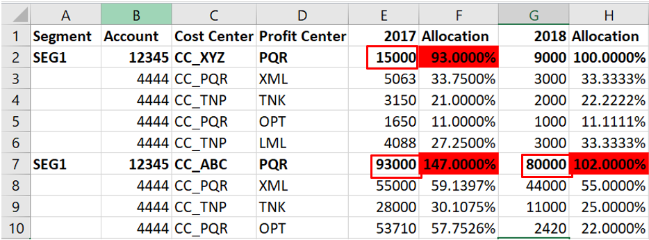
1. As per screen shot if Red color highlighted cell system found then immediate adjacent cell (prior to formatted cell) should also fill with Red color.

2. Example : Cell E2 is not color currently but F2 is colored.

3. In other way if total of 12345 account is not match with 4444 account then 12345 account total should be fill with color.

Is there any way out using macro if this is possible. Or if any excel formula can fulfill this requirement please help on the same.

PS

[former_member186338]

Sample formula for conditional formatting to look on the value of the next cell in the row:

=AND(INDIRECT("rc[1]",FALSE)>=1,INDIRECT("rc[1]",FALSE)<=1.001)

rc[1] - reference to next cell in the row

[former_member186338]

For conditional formatting you can use formula ("Use a formula to determine...")

And you can use conditional formatting for column E with formula looking for the value in column F.

Easy!

[former_member186338]

Please explain: "In other way if total of 12345 account is not match with 4444 account then 12345 account total should be fill with color."

Please show the formula used to perform conditional formatting of F2!

And what do you have in F2? Local member?

[former_member394086]

Hi Vadim,

Please find attached conditional formatting which I used for F2.

Also I mean 12345 is a sender account. which is having total 15000. 4444 is the receiver account for which its total also should be 15000. But if %age not showing 100% then its total also definitely will not match. So I am either looking for solution by compairing this total or by using existing conditional formatting and then color expected row.

[former_member186338]

Sorry, you are not reading my posts to the end:

"And what do you have in F2? Local member?"

[former_member394086]

Yes all the four column i.e. E, F , G and H are local members.

[former_member186338]

Can you provide local member formulas?

Strange to have local member in E and G... I am lost with your report!

[gcybill]

Please refer to this:

https://www.excel-university.com/excel-conditional-formatting-based-on-another-cell/

You can also combine with EPM formatting feature.