- SAP Community
- Products and Technology
- Technology
- Technology Q&A
- Comparing multiple columns and cumulative sum at m...
- Subscribe to RSS Feed
- Mark Question as New
- Mark Question as Read
- Bookmark
- Subscribe
- Printer Friendly Page
- Report Inappropriate Content
Comparing multiple columns and cumulative sum at max valued cell in Webi
- Subscribe to RSS Feed
- Mark Question as New
- Mark Question as Read
- Bookmark
- Subscribe
- Printer Friendly Page
- Report Inappropriate Content
on 04-04-2019 3:16 PM
Hi All,
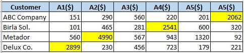
We have a requirement where we need to identify which all values are greater than 200 for each row, and then all those values need to be summed up and displayed at that cell which has the highest value among all columns per row. The examples are shown below.
This is the current report:

Expected report:
All I could think of right now is, that we have to implement ifelsethen logic to identify the maximum value of columns per row. Any suggestions would be much appreciated.
Thanks
- SAP Managed Tags:
- SAP BusinessObjects - Web Intelligence (WebI)
Accepted Solutions (1)
Accepted Solutions (1)
- Mark as New
- Bookmark
- Subscribe
- Subscribe to RSS Feed
- Report Inappropriate Content
Try this:
Create a formula to select the value which are greater than or equal to 200 first:
[v_lowhoigh] = =If(Not([Value]=Min([Value]) In ([Customer])) And ([Value]>=200)) Then 1 Else 0
Now use the below formula in your cross tab table:
=If(Not([Value]=Max([Value]) In ([Customer]))) Then [Value] Else(Sum([Value] Where([v_lowhigh]=1)) In ([Customer]) - Sum([Value] Where([v_lowhigh]=0) ) )

You can also do a conditional formatting to show the highest value cell which is showing the cumulative sum.
You must be a registered user to add a comment. If you've already registered, sign in. Otherwise, register and sign in.
Answers (0)
- Harnessing the Power of SAP HANA Cloud Vector Engine for Context-Aware LLM Architecture in Technology Blogs by SAP
- SAP Analytics Cloud Planning - Converting data in Technology Blogs by SAP
- Workload Analysis for HANA Platform Series - 1. Define and Understand the Workload Pattern in Technology Blogs by SAP
- Boosting Benchmarking for Reliable Business AI in Technology Blogs by SAP
- What's New in the Newly Repackaged SAP Integration Suite, advanced event mesh in Technology Blogs by SAP
| User | Count |
|---|---|
| 89 | |
| 10 | |
| 9 | |
| 9 | |
| 9 | |
| 6 | |
| 6 | |
| 5 | |
| 5 | |
| 4 |
You must be a registered user to add a comment. If you've already registered, sign in. Otherwise, register and sign in.